SAE 2011-01-0001

ABSTRACT

Advanced High Strength Steels (AHSS) have been implemented in the automotive industry to balance the requirements for vehicle crash safety, emissions, and fuel economy. With lower ductility compared to conventional steels, the fracture behavior of AHSS components has to be considered in vehicle crash simulations to achieve a reliable crashworthiness prediction. Without considering the fracture behavior, component fracture cannot be predicted and subsequently the crash energy absorbed by the fractured component can be over-estimated. In full vehicle simulations,failure to predict component fracture sometimes leads to less predicted intrusion. In this paper, the feasibility of using computer simulations in predicting fracture during crash deformation is studied. Three material fracture models,MAT_24, MAT_123, and MMC fracture model, available in LS-Dyna? finite element analysis code are adopted to simulate the fracture behavior of two dual phase (DP) grades,i.e., DP590 and DP780 steels. To provide test data for the model validations, components made of DP590 and DP780were fabricated and tested with axial crush and three-point bending loading conditions. During the simulation, forming simulation results such as plastic strains, thinning and damage parameters were mapped to the crash models as initial conditions in crash simulations so that the sensitivity of the forming effect on fracture modeling could be studied. The predicted crush force and crush mode were then compared to those from the component crush tests. The capability of the three material fracture models for fracture prediction was assessed and the results are discussed.

INTRODUCTION

AHSS, including Dual Phase (DP) and Transformation Induced Plasticity (TRIP) steels, have improved crash energy absorption capability when compared to conventional mild steels. In recent years, AHSS have been widely accepted as the material of choice to balance vehicle weight, vehicle crash, durability and NVH performance. According to a study on North American light vehicle metallic material trends by Ducker Worldwide [1], AHSS will grow 10% annually and reach over 204 kg per vehicle by 2020. It is expected that AHSS will be used approximately 3 times more frequently than current levels by 2020 in North American light vehicle body structures.

While the increased usage of AHSS resulted in weight savings, one performance parameter to be studied is fracture during a vehicle crash event. Fracture that was rarely observed in crash tests a decade ago occurs more frequently in AHSS parts due to the relatively lower ductility compared to conventional mild steels. To appropriately apply AHSS and maximize weight reduction potential, it is important to develop the capability to predict the fracture behavior correctly in crash simulations and to accurately assess designs in the vehicle development process.

Although crash simulations have been successfully used during vehicle development to assess the energy absorption capability of the vehicle, continuous improvements in many areas are still required to further improve the quality of the crash simulations. One of those areas is the prediction of the fracture behavior of structural components under different crash loadings. Crash simulations that do not take into

account the fracture behavior may overstate the load-carrying

Fracture Modeling of AHSS in Component Crush Tests

2011-01-0001

Published 04/12/2011

Guofei Chen and Ming F. Shi

United States Steel Corporation

Tau Tyan

Ford Motor Company

Copyright ? 2011 SAE International

doi:10.4271/2011-01-0001

SAE Int. J. Mater. Manuf. | Volume 4 | Issue 1

1

capacity and the absorbed energy of a structural component. The application of AHSS makes fracture prediction more important since those materials can be relatively prone to fracture during crash deformation.

Many original equipment manufacturers (OEMs) have been using the material failure model CrachFEM linked to various explicit dynamic finite element method (FEM) programs to predict ductile and shear fracture [2, 3]. In this study, material fracture models available in the widely used explicit FEM code LS-Dyna? are adopted to simulate the fracture behavior of two of the most widely used AHSS grades, i.e., DP590 and DP780 steels in crush loadings. Three material models, i.e., *MAT_PIECEWISE_LINEAR_PLASTICITY (MAT_24) with a maximum equivalent plastic strain as the failure criterion,

*MAT_MODIFIED_PIECEWISE_LINEAR_PLASTICITY (MAT_123) with a major in-plane strain or the major principal strain as the failure criterion, and the newly modified Mohr-Coulomb (MMC) fracture model [4] with stress triaxiality dependent equivalent plastic strains as the failure criterion, are investigated. The predicted crush force, crush and fracture modes are then compared to those from the component axial crush tests and three-point bending crush tests. The capability of the three material fracture models for the fracture prediction is assessed and the results are discussed in the paper.

MATERIAL MODELS

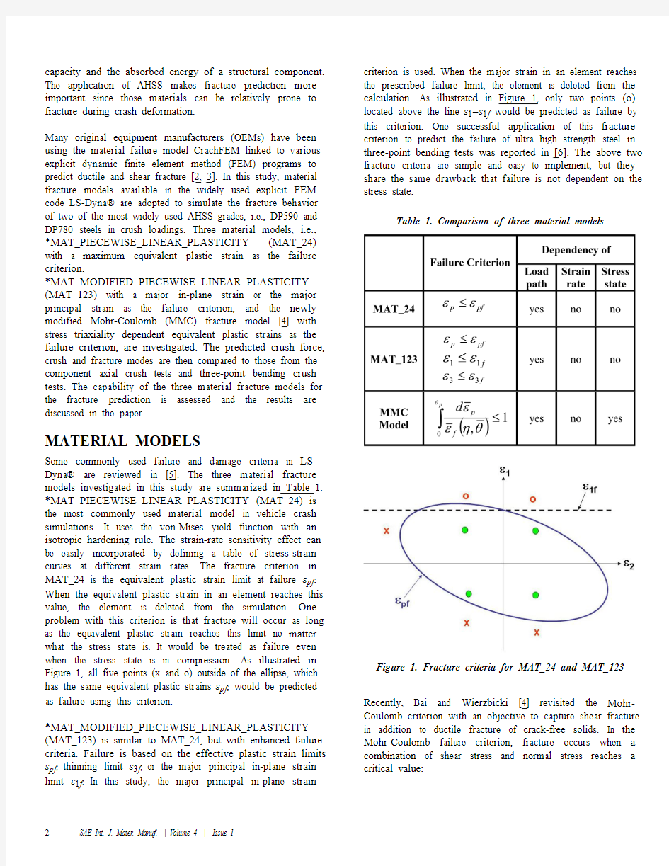
Some commonly used failure and damage criteria in LS-Dyna? are reviewed in [5]. The three material fracture models investigated in this study are summarized in Table 1. *MAT_PIECEWISE_LINEAR_PLASTICITY (MAT_24) is the most commonly used material model in vehicle crash simulations. It uses the von-Mises yield function with an isotropic hardening rule. The strain-rate sensitivity effect can be easily incorporated by defining a table of stress-strain curves at different strain rates. The fracture criterion in MAT_24 is the equivalent plastic strain limit at failure εpf. When the equivalent plastic strain in an element reaches this value, the element is deleted from the simulation. One problem with this criterion is that fracture will occur as long as the equivalent plastic strain reaches this limit no matter what the stress state is. It would be treated as failure even when the stress state is in compression. As illustrated in Figure 1, all five points (x and o) outside of the ellipse, which has the same equivalent plastic strains εpf, would be predicted as failure using this criterion.

*MAT_MODIFIED_PIECEWISE_LINEAR_PLASTICITY (MAT_123) is similar to MAT_24, but with enhanced failure criteria. Failure is based on the effective plastic strain limits εpf, thinning limit ε3f, or the major principal in-plane strain limit ε1f. In this study, the major principal in-plane strain criterion is used. When the major strain in an element reaches the prescribed failure limit, the element is deleted from the calculation. As illustrated in Figure 1, only two points (o) located above the line ε1=ε1f would be predicted as failure by this criterion. One successful application of this fracture criterion to predict the failure of ultra high strength steel in three-point bending tests was reported in [6]. The above two fracture criteria are simple and easy to implement, but they share the same drawback that failure is not dependent on the stress state.

Table 1. Comparison of three material models

Figure 1. Fracture criteria for MAT_24 and MAT_123 Recently, Bai and Wierzbicki [4] revisited the Mohr-Coulomb criterion with an objective to capture shear fracture in addition to ductile fracture of crack-free solids. In the Mohr-Coulomb failure criterion, fracture occurs when a combination of shear stress and normal stress reaches a critical value:

SAE Int. J. Mater. Manuf. | Volume 4 | Issue 1 2

(1)

where C 1 and C 2 are material constants. Bai and Wierzbicki [4] modified Equation (1) by transforming it from the stress-

based form to a mixed strain-stress space of (

, , ). The

modified Mohr-Coulomb fracture criterion is described as:

(2)

where is the equivalent plastic strain at

fracture, is stress triaxiality defined by the ratio of the mean stress to the von Mises equivalent

stress, ,

and is the normalized Lode angle parameter. c 1, c 2 and c 3 are fracture-related material parameters. A and n are material constants described in the modified Swift law in the uniaxial tension

test:

(3)

For sheet metals deformed in the plane stress state, can be eliminated, and the 3-D MMC criterion described in Equation (2) can be simplified o a 2-D fracture criterion defined in the

space of and . Figure 2 shows a typical MMC fracture locus under the plane stress condition and the corresponding material characterization tests used to calibrate the material parameters [7]. Since the model has three parameters, a minimum of three tests are needed to calibrate the parameters. It is recommended [7] that the equi-biaxial punch fracture test, the transverse plane strain fracture test and the shear fracture test be used for parameter calibrations. These tests maintain a constant stress triaxiality evolution until the point of fracture and allow for the direct measurement of the

strain at fracture.

Figure 2. A typical MMC fracture locus and the material

characterization tests In addition to the fracture locus, a damage parameter D is defined to specify the damage evolution rule when the material is deformed under non-proportional loadings. It is assumed that the damage parameter D is accumulated as a linear function of the increment of the equivalent plastic strain normalized with respect to the current value of the fracture locus

under proportional loading:

(4)

Fracture initiates when D reaches the critical value Dc ,usually taken as unity, and the corresponding element is deleted. The MMC model is currently implemented in LS-Dyna? with a user subroutine using material model card *MAT_USER_DEFINED_MATERIAL_MODELS. The MMC fracture model has been successfully applied to the shear fracture prediction that occurs on the bending radius when AHSS material is drawn and bent over the radius during forming [8, 9].

The same parameters of the MMC model used in [9] were adopted for the DP780 material. For DP590 material, various tests were performed at United States Steel Corporation's Automotive Center and calibrated parameters were also obtained. The fracture locus in the plane stress condition is shown in Figure 3 for both DP590 and DP780. The characterized material constants for the MMC model and tensile properties are shown in the Table 2.

SAE Int. J. Mater. Manuf. | Volume 4 | Issue 13

Figure 3. MMC fracture locus for DP590 and DP780

steels

Table 2. Material tensile properties and MMC constants

CRUSH TESTS

Axial and three-point bending crush tests were conducted to obtain test data for the model validations. Components with a 12-sided cross-section were fabricated by press-forming laser-welded conical tubes around a 12-sided mandrel die [10]. The bend radii for the corners are about 3 mm. The 12-sided design demonstrated superior axial crush energy absorption capability to other geometries in previous studies [10, 11].

The set-up for the axial crush for 1.5-mm DP590 is shown in Figure 4(a). The test sample was welded to a base plate and placed on a VIA sled vehicle. The sled vehicle was accelerated to 6.7 m/sec (15 mph) before crashing into a rigid wall. The total weight of the sled-vehicle is 1362 kg.Accelerometers were attached to the sled to record deceleration, and crush force data can be obtained by multiplying deceleration by the sled mass or by directly using the reaction force data recorded in the load cells installed on

the rigid wall. Photos and videos were taken during the crush using high-speed video cameras. Figure 4(b) shows that cracks developed after the initial 3 folds on the 12-sided sample and propagated by tearing along the corners.Figure 5(a) shows the set-up for the quasi-static bending test on 1.6-mm DP780. The span length between two supports is 560 mm. A cylindrical punch with a diameter of 50.8 mm hit the sample at the center at a speed of 0.423 mm/sec (1.0 inch/minute). The reaction forces were measured with three load cells located at the punch and each support. A string potentiometer was used to measure the displacement of the punch. Photos and videos were taken during the crush using high-speed video cameras. Cracks were observed at the

corners, as shown in Figure 5(b).

(a). Axial crush test set-up

(b). Cracked 12-sided sample

Figure 4. Axial crush test at 6.7 m/sec on DP590

SAE Int. J. Mater. Manuf. | Volume 4 | Issue 1

4

(a). Quasi-static bending crush test set-up

(b). Cracked sample after bending crush test Figure 5. Three-point bending crush test on DP780

SIMULATIONS AND VALIDATIONS

Before the crush simulation, the incremental forming simulation was performed using LS-Dyna?, and the forming simulation results were then mapped to the crush simulation model to account for the forming effects. For simplicity, the isotropic hardening yield criterion is used during forming.For the MMC model, damage parameter D accumulated during forming was also mapped to the crash model in addition to other forming simulation results including thickness, equivalent plastic strain and strain components.Figure 6 shows the damage predicted from the forming simulation using the MMC model, with the damage localized mainly around the corners.

Belytschko-Tsay (type 2) shell elements with five through thickness integration points were utilized in all simulations.Figure 7 compares the crush forces predicted by the MMC model for different through thickness integration points with the bending test results. It is seen that five through thickness integration points are accurate enough while maintaining

good computational efficiency.

(a). Damage on the bending crush sample

(b). Damage on the axial crush sample

Figure 6. Damage predicted from the forming simulation

Figure 7. Comparison of through thickness integration

points The mesh size dependency is a common issue in fracture prediction where a crack is initiated and propagated by element deletion [12]. The finite element mesh should be fine enough to capture material localization arising before fracture. A practical approach to minimize the effect of mesh size is to maintain an approximate same length scale in simulations as that used in calibrations of the fracture model parameters. In this study, the 1.0-mm mesh size was used in all simulations, which is consistent with the length scale used in the MMC model parameters calibration [9]. The sensitivity of mesh sizes on fracture predictions can be found in Figure 8.

SAE Int. J. Mater. Manuf. | Volume 4 | Issue 15

When considering fracture prediction in full vehicle crash model, “selective mass scaling” can be adopted and applied to components with very small element sizes. The “selective mass scaling” will allow the global time step in the full vehicle not to be affected by the local time step in the selective components with small mesh sizes.

For the dynamic axial crush, the strain rate is generally over 100 /s. The effect of strain rates on the fracture locus or failure limit for AHSS steels is still an on-going research subject with limited available test data. The data in [13] for AISI 4340 steel and other metals show that the strain rate and temperature effects are less important than the stress state effect. Therefore, the strain rate effect on fracture behavior was not considered in dynamic axial crush simulations in this study.

As a model validation, a uniaxial tensile test on DP590 was simulated with the MMC model. Figure 9 compares the simulation results with the test for the force-displacement curve and fracture mode. The displacement and load drop at

fracture from the simulation match the test well.

Figure 8. Effect of mesh size on fracture mode

Figure 9. Simulation of tensile test on DP590 using

MMC model

BENDING CRUSH

The quasi-static three-point bending test on DP780 was simulated using the three material models. The simulated fracture mode and force-displacement curves are compared in Figures 10 and 11. All three material models are capable of predicting the fracture locations at the corners as observed in the tests shown in Figure 5(b) when the forming effect is considered in the crush simulations, and the force-displacement curves from the simulations match the tests well. This is not surprising because all three material models use the same von-Mises yield criterion with differences only in the fracture criteria. In the bending crush mode, the materials around the buckle area are deformed under approximately plane strain state, which allows both MAT_24and MAT_123 to simulate the fracture well although the failure strain limits are constant and independent of the stress state.

The forming effects are demonstrated in Figures 10 and 11using the MMC model. The predicted peak load is about 10%lower if the forming effects are not included in the crush simulation. However, the initial damage from the forming process contributed little to fracture in the bending crush, as shown in Figures 10(c) and (d) with similar fracture locations and crack sizes. This phenomenon can be explained in Figure 12, which shows the development of the damage parameter D for one failed element at the corner during the bending crush.Since the corners were formed by bending, the upper surface of the element was in tension and the lower surface in compression, and the forming induced damage was mainly on the upper surface of the element with little damage shown on the lower surface of the element. During the bending crush,however, damage developed quickly on the lower surface since the lower surface was in tension. Fracture initiated from the lower surface when the damage parameter D reached the critical value of one. As shown in Figure 12, the fracture initiation from the lower surface delays only a little bit if the

SAE Int. J. Mater. Manuf. | Volume 4 | Issue 1

6

forming effect is not included in the crush simulation since

there is little damage in the lower surface from forming.

Figure 10. Comparison of fracture mode in bending

crush

Figure 11. Comparison of crush force in bending crush

Figure 12. Development of the Damage Parameter D

AXIAL CRUSH

The deformation mode in axial crush is more complicated.The side walls of the crushing components bend in a plane strain condition, while the corners are approximately in shear mode. Figures 13 and 14 show the simulated fracture mode and force-displacement curves for the 6.7 m/sec (15 mph)axial crush test on DP590 using the three material models mentioned above.

When compared to the fracture mode shown in Figure 4(b),the MMC model and MAT_123 are able to predict fracture after 3 folds and tearing along the corners thereafter, while MAT_24 predicts fracture at the beginning of the crush before the folds are developed. This is the shortcoming of MAT_24, which uses a constant equivalent plastic strain as the fracture limit regardless of whether the deformation is in tension or compression. MAT_123 model shows the improvement due to the fact that the major principal strain instead of the equivalent strain is used as the fracture limit.The force-displacement curves predicted using both MAT_123 and the MMC models also agreed well with the test results as shown in Figure 14. The predictions of initial crush load from simulations are lower than that of the test.The discrepancy might be attributed to the welding of the components. The heat generated through the welding process may have affected the property of the material. The change of material property due to welding was not considered in the models. A detailed study will be conducted in the next phase of the project to further investigate the discrepancy.

As shown in Figures 13 (c) and (d) using the MMC model,the initial damage from the forming process does show some effect on the fracture mode in the axial crush. When the forming effect is not considered in the crush simulation, the tearing mode could not be predicted, and the crush response is softer with about 6% larger crush distance.

SAE Int. J. Mater. Manuf. | Volume 4 | Issue 17

Although MAT_123 successfully captures the overall fracture mode in the axial crush, it predicts extensive fracture at all corners of the front end, as shown in Figure 15(a), which is in contradictory to the test results as shown in Figure 4(b). That is because the principal fracture strain used in MAT_123 is determined from the plane strain and the principal strain predicted in the shear mode at the corners is higher than the fracture strain. For the MMC fracture locus, however, the fracture limit is much higher when the material deforms in shear mode, as shown in Figure 3. Figure 15(b) shows the MMC model predicts only limited fracture at the front end when the crush started.

Overall, the MMC model performed well in capturing the fracture mode in both bending and axial crushes since its fracture locus is stress state dependent, but at a cost of 30%more CPU time than MAT_24 and MAT_123. MAT_123gave a good prediction in the bending crush and reasonably good prediction in the axial crush. MAT_24 could not capture the fracture mode in the axial crush because the failure criterion's intrinsic deficiency and should be used with caution for fracture prediction in structures with complex

states of stress or involved in complicated loading paths.

Figure 13. Comparison of fracture mode in axial crush

Figure 14. Comparison of crush force in axial crush

Figure 15. Deformation at the front end

CONCLUSIONS

Three material fracture models of axial and bending crush were investigated against actual test data. The following conclusions can be drawn from this study:

? The MMC model performed well in fracture predictions for both the bending and axial crush tests conducted in this study.? With a simple failure criterion and computational efficiency, MAT_123 gave a good prediction in the bending crush and a reasonably good prediction in the axial crush.? MAT_24 could not capture the fracture mode in the axial crush and should be avoided in the fracture prediction for deformation with complicated loading paths.

? For bending crush, the consideration of forming results in the crush simulation had no effect on the fracture mode but some effect on crash force predictions. For the axial crush simulation, the forming effect must be considered in the crush simulation since the forming results had a significant influence on the fracture mode and the crash force predictions.

SAE Int. J. Mater. Manuf. | Volume 4 | Issue 1

8

NEXT STEPS

Several topics can be investigated further in the future to expand the understanding and knowledge of fracture modeling. These factors include:

? The effect of material anisotropy due to rolling process.? Stress relaxation of the component after forming.

? Failure prediction for components with holes and slots.? Comparison of prediction with other failure constitutive models, such as those from CrachFEM and other newly developed constitutive models.

REFERENCES

1. Schultz, R.A. and Abraham, A.K., “Metallic Material Trends for North American Light Vehicles,” 2009 Great Design in Steel Seminar sponsored by American Iron and Steel Institute (AISI), Livonia, MI, May 2009.

2. Lanzerath, H., Bach, A., Oberhofer, G. and Gese, H.,“Failure Prediction of Boron Steels in Crash,” SAE Technical Paper 2007-01-0989, 2007, doi:10.4271/2007-01-0989.

3. Werner, H., Hooputra, H., Weyer, S. and Gese, H.,“Applications of Phenomenological Failure Models in Automotive Crash Simulations,” VIII International Conference on Computational Plasticity, COMPLAS VIII, Barcelona, 2005.

4. Bai, Y. and Wierzbicki, T., “A New Model of Metal Plasticity and Fracture with Pressure and Lode Dependence,”International Plasticity, 24, 6 (2008), pp. 1071-1096.

5. Du Bois, P.A., Kolling, S., Feucht, M., Haufe, A., “A Comparative Review of Damage and Failure Models and a Tabulated Generalization,” 6th European LS-DYNA User's Conference, Gothenburg, Sweden, May 2007.

6. Wang, H., Sivasamy, S., and Schroter, M., “Material Failure Approaches for Ultra High Strength Steel,” LS-Dyna Anwenderforum, Ulm, Germany, 2006.

7. Luo, M. and Wierzbicki, T., “Ductile Fracture Calibration and Validation of Anisotropic Aluminum Sheets,” in Proceedings of 2009 SEM Annual Conference and Exposition on Experimental and Applied Mechanics, Society of Experimental Mechanics, pp. 402-413, Albuquerque, NM, 2009.

8. Chen, X., Shi, M.F., Shih, H-C., Luo, M. and Wierzbicki, T., “AHSS Shear Fracture Predictions Based on a Recently Developed Fracture Criterion,” SA E Int. J. Mater. Manuf.

3(1):723-731, 2010, doi:10.4271/2010-01-0988.

9. Luo, M., Chen, X.M., Shi, M.F. and Shih, H.C.,“Numerical Analysis of AHSS Fracture in a Stretch-bending Test,” NUMIFORM 2010: Proceedings of the 10th International Conference on Numerical Methods in Industrial Forming Processes Dedicated to Professor O. C. Zienkiewicz (1921-2009). AIP Conference Proceedings, Vol. 1252, pp. 455-463, 2010.

10. Chen, G., Link, T.M., Shi, M.F., Tyan, T., Gao, R. and McKune, P.M., “Axial Crash Testing and Finite Element Modeling of A 12-Sided Steel Component,” SA E Int. J. Mater. Manuf.3(1):162-173, 2010, doi:

10.4271/2010-01-0379.

11. Chen, G., Shi, M.F. and Tyan, T., “Cross-Section Optimization for Axial and Bending Crashes Using Dual Phase Steels,” SAE paper 2008-01-1125, SAE International Journal of Materials & Manufacturing, Vol.1, pp. 537-547, April 2009.

12. Li, Y.N., Karr, D.G., and Wang, G., “Mesh Size Effects in Simulating Ductile Fracture of metals,” 10th International Symposium on Practical Design of Ships and Other Floating Structures, Houston, Texas, 2007.

13. Johnson, G.R. and Cook, W.H., “Fracture Characteristics of Three Metals Subjected to Various Strains, Strain Rates, Temperatures and Pressures,” Engineering Fracture Mechanics, Vol. 21, No. 1, pp. 31-48, 1985. CONTACT INFORMATION

Dr. Guofei Chen

Product Application Engineer - CAE

United States Steel Corporation - Automotive Center

5850 New King Ct, Troy, MI, USA

gchen@https://www.sodocs.net/doc/226964986.html,

ACKNOWLEDGMENTS

The authors would like to acknowledge Dr. Xinhai Zhu of Livermore Software Technology Corporation (LSTC) for implementing the MMC model in LS-Dyna and consulting on using the new model; Dr. Aleksy Konieczny of United States Steel Corporation for conducting material characterization tests on DP590 and providing the data used in the simulations; the colleagues at Ford Safety Laboratory for conducting the crush tests; and Todd Link of United States Steel Corporation for proofreading the paper. DISCLAIMER

The material in this paper is intended for general information only. Any use of it in relation to specific applications should be based on independent examination and verification of its unrestricted availability for such use and determination of suitability for the application by professionally qualified personnel. No license under any patents or other proprietary interest is implied by the publication of this paper. Those making use of or relying upon this material assume all risks and liabilities arising from such use or reliance.

SAE Int. J. Mater. Manuf. | Volume 4 | Issue 19

标准之各种硬度单位换算表以及水质硬度范围

碱度：把天然水经处理过的水的PH降低到相应于纯CO2水溶液的PH值所必须中和的水中强碱物种的总含量。按这个定义，碱度由强酸（盐酸或硫酸）滴定至终点，单位为ep/L. 硬度：通常说的总硬度指水中Ca2+,Mg2+的总量，这是因为其他离子的总含量远小于二者的含量，因此不予考虑。只有在其他量子含量很高时才考虑，其对硬度的影响。水中的阳离子（除H+外）一般也碳酸盐，重碳酸盐，硫酸盐及氯化物等形式存在。 硬度可以分为暂时硬度，永久硬度个负硬度等类型。 暂时硬度：又称碳酸盐硬度，指水中钙，镁的碳酸盐的含量，因天然水中碳酸盐含量很低，只有在碱性水中才存在碳酸盐。故暂时硬度一般是指水中重碳酸盐的含量，水在煮沸时其中的重碳酸盐分解出碳酸盐沉淀。常用的硬度单位是毫摩尔/升（mmol/L） 永久硬度：又称非碳酸盐硬度，主要指水中钙，镁的氯化物.硫酸盐的含量，之外尚有少量的钙.镁硝酸盐.硅酸盐等盐类，在常压9体积不变）情况下加热，这些盐类不会析出沉淀。常用的硬度单位是毫摩尔/升（mmol/L） 负硬度：指水中钾.纳的碳酸盐.重碳酸盐及氢氧化物的含量，又称为纳盐硬度。当水的总碱度大于总硬度时，就回出现负硬度。负硬度可以消除水的永久硬度，负硬度不能与永久硬度共存。常用的硬度单位是毫摩尔/升（mmol/L） 碱度和硬度是水的重要参数，二者之间的关系有以下三种情况： （1）总碱度〈总硬度，此时，水中有永久硬度和暂时硬度，无钠盐（负）硬度，则： 总硬度—总碱度=永久硬度 总碱度=暂时硬度 （2）总碱度〉总硬度，水中无永久硬度，而存在暂时硬度和钠盐硬度，则： 总硬度=暂时硬度 总碱度—总硬度=钠盐硬度（负硬度） （3）总碱度=总硬度，水中没有永久硬度和钠盐硬度，只有暂时硬度，则： 总硬度=总碱度=暂时硬度 1 / 1

硬度换算表、公差、表面粗糙度值(打印清晰版)

HRA HRC HRA HRC HRA HRC HRA HRC 86.6 70.0103778.555.059937070.540.037726928.027486.3 69.5101778.254.558936570.339.537226627.527186.1 69.099777.954.057936070.039.036726327.026885.8 68.597877.753.557035538.536226026.526485.5 68.095977.453.056135038.035125726.026185.2 67.594177.152.555134537.535225425.525885.0 67.092376.952.054334137.034725125.025584.7 66.590676.651.553433636.534224824.525284.4 66.088950176.351.052533236.033824524.024984.1 65.587249476.150.551732735.533324223.524683.9 65.085648875.850.050932335.032924023.024383.6 64.584048175.549.550131834.532423722.524083.3 64.082547475.349.049331434.032023422.023783.1 63.581046875.048.548531033.531623221.523482.8 63.079546174.748.047830633.031222921.023182.5 62.578045574.547.547030232.530822720.522982.2 62.076644974.247.046329832.030422520.022682.0 61.575244273.946.545629431.530022219.522381.7 61.073943673.746.044929131.029622019.022181.4 60.572643073.445.544328730.529221818.521881.2 60.071342473.245.043628330.028921618.021680.9 59.570041872.944.542928029.528521417.521480.6 59.068841372.644.042327629.028121117.021180.3 58.567640772.443.541727328.527880.1 58.066440172.143.041179.8 57.565339671.842.540579.5 57.064239171.642.039979.3 56.563138571.341.539379.0 56.062038071.141.038878.755.560937570.840.5382黑色金属材料 硬度值换算表 布氏硬度 HB 洛氏硬度 维氏硬度HV 布氏硬度HB 洛氏硬度维氏硬度HV 布氏硬度HB 维氏硬度HV 注:1.布氏硬度:主要用来测定铸件、锻件、有色金属制件、热轧坯料及退火件的硬度,测定范围≯HB450。 2.洛氏硬度:HRA 主要用于高硬度试件,测定硬度高于HRC67以上的材料和表面硬度,如硬质合金、氮化钢等，测定范围HRA>70。HRC 主要用于钢制件(如碳钢、工具钢、合金钢等）淬火或回火后的硬度测定,测定范围HRC20~67。 3.维氏硬度:用来测定薄件和钢板制件的硬度,也可用来测定渗碳、氰化、氮化等表面硬化制件的硬度。 洛氏硬度维氏硬度HV 布氏硬度HB 洛氏硬度

硬度值对照表

BUEHLER?Tables for Knoop and Vickers Hardness Numbers

Table of Contents Load 5 gf (0.005kgf) . . . . . . . . . . . . . . . . . . . . . . . . . . . . . . . . . . . . . . . . . . . . . . . . . . . . . . . . . . . . . . . . . . . . . . . . .1 Load 10 gf (0.01kgf) . . . . . . . . . . . . . . . . . . . . . . . . . . . . . . . . . . . . . . . . . . . . . . . . . . . . . . . . . . . . . . . . . . . . . . . . . .3 Load 25 gf (0.025kgf) . . . . . . . . . . . . . . . . . . . . . . . . . . . . . . . . . . . . . . . . . . . . . . . . . . . . . . . . . . . . . . . . . . . . . . . .5 Load 50gf (0.05kgf) . . . . . . . . . . . . . . . . . . . . . . . . . . . . . . . . . . . . . . . . . . . . . . . . . . . . . . . . . . . . . . . . . . . . . . . . . .8 Load 100gf (0.1kgf) . . . . . . . . . . . . . . . . . . . . . . . . . . . . . . . . . . . . . . . . . . . . . . . . . . . . . . . . . . . . . . . . . . . . . . . . .12 Load 200gf (0.2kgf) . . . . . . . . . . . . . . . . . . . . . . . . . . . . . . . . . . . . . . . . . . . . . . . . . . . . . . . . . . . . . . . . . . . . . . . . .16 Load 300gf (0.3kgf) . . . . . . . . . . . . . . . . . . . . . . . . . . . . . . . . . . . . . . . . . . . . . . . . . . . . . . . . . . . . . . . . . . . . . . . . .17 Load 500gf (0.5kgf) . . . . . . . . . . . . . . . . . . . . . . . . . . . . . . . . . . . . . . . . . . . . . . . . . . . . . . . . . . . . . . . . . . . . . . . . .24 Load 1000gf (1kgf) . . . . . . . . . . . . . . . . . . . . . . . . . . . . . . . . . . . . . . . . . . . . . . . . . . . . . . . . . . . . . . . . . . . . . . . . .29 Load 2000gf (2 kgf) . . . . . . . . . . . . . . . . . . . . . . . . . . . . . . . . . . . . . . . . . . . . . . . . . . . . . . . . . . . . . . . . . . . . . . . . .36 Load 5kgf . . . . . . . . . . . . . . . . . . . . . . . . . . . . . . . . . . . . . . . . . . . . . . . . . . . . . . . . . . . . . . . . . . . . . . . . . . . . . . . . . .44 Load 10kgf . . . . . . . . . . . . . . . . . . . . . . . . . . . . . . . . . . . . . . . . . . . . . . . . . . . . . . . . . . . . . . . . . . . . . . . . . . . . . . . . .46 Load 20kgf . . . . . . . . . . . . . . . . . . . . . . . . . . . . . . . . . . . . . . . . . . . . . . . . . . . . . . . . . . . . . . . . . . . . . . . . . . . . . . . . .48 Load 30kgf . . . . . . . . . . . . . . . . . . . . . . . . . . . . . . . . . . . . . . . . . . . . . . . . . . . . . . . . . . . . . . . . . . . . . . . . . . . . . . . . .50 Load 50kgf . . . . . . . . . . . . . . . . . . . . . . . . . . . . . . . . . . . . . . . . . . . . . . . . . . . . . . . . . . . . . . . . . . . . . . . . . . . . . . . . .52

水的硬度单位换算Word版

水的硬度 水质硬度单位换算 电导率 电导率与水的硬度 软水与硬水 水分为软水、硬水，凡不含或含有少量钙、镁离子的水称为软水，反之称为硬水。水的硬度成份，如果是由碳酸氢钠或碳酸氢镁引起的，系暂时性硬水（煮沸暂时性硬水，分解的碳酸氢钠，生成的不溶性碳酸盐而沉淀，水由硬水变成软水）；如果是由含有钙、镁的硫酸盐或氯化物引起的，系永久性硬水。依照水的总硬度值大致划分，总硬度0-30ppm称为软水，总硬度60ppm以上称为硬水，高品质的饮用水不超过25ppm，高品质的软水总硬度在10ppm以下。在天然水中，远离城市未受污染的雨水、雪水属于软水；泉水、溪水、江河水、水库水，多属于暂时性硬水，部分地下水属于高硬度水。 一百多年来，科学技术极大地推动近代工业、现代工业、当代工业高速发展，渐渐改善人类生活条件的同时，无处不在的化学技术、工业污染极大地破坏着地球环境的固有平衡，使水资源遭受着严重的污染，水，早已不在是几百年前大都可以直接饮用的水，而是含有许多悬浮物、胶体、以及钙、镁等有害重金属离子、病菌。由于家庭用水量的95％以上属非饮用性生活用水，因此，品质不良的水，不仅危害着人体健康，而且危害着涉水性日常生活、涉水性家庭器具。

水质硬度单位的换算表

说明:表中所列每升所含毫克当量的数值,按照德国和苏联的标准,1度相当于每L水中含0.35663毫克当量的CaO,或每L水中含10mg的CaO.按照法国的标准,1 度相当于每L水中含0.19982毫克当量的CaCO 3,或每L水中含10mg的CaCO 3 .按照 美国的标准,1度相当于每L水中含0.01998毫克当量的CaCO 3 ,或每L水中含1mg的 CaCO 3.按照英国的标准,1度相当于每L水中含0.28483毫克当量的CaCO 3 ,或0.7L 水中含10mg的CaCO 3.

2013年国家标准各种硬度值换算表

国家标准各种硬度值换算表 Steel Rockwell Rockwell Superficial Vickers Brinell Shore HRA HRB HRC HRD 15N 30N 45N HV HB HS 60kgf 100kgf 150kgf 100kgf 15kgf 30kgf 45kgf 50kgf 3000kgf jis 85.6 68.0 76.9 93.2 84.4 75.4 940 97.6 85.3 67.5 76.5 93.0 84.0 74.3 920 96.4 85.0 67.0 76.1 92.9 83.6 74.2 900 95.2 84.7 66.4 75.7 92.7 83.1 73.6 880 94.0 84.4 65.9 75.3 92.5 82.7 73.1 860 92.8 84.1 65.3 74.8 92.3 82.2 72.2 840 91.5 83.8 64.7 74.3 92.1 81.7 71.8 820 90.2 83.4 64.0 73.8 91.8 81.1 71.0 800 88.9 83.0 63.3 73.3 91.5 80.4 70.2 780 87.5 82.6 62.5 72.6 91.2 79.7 69.4 760 86.2 82.2 61.8 72.1 91.0 79.1 68.6 740 84.8 81.8 61.0 71.5 90.7 78.4 67.7 720 83.3 81.3 60.1 70.8 90.3 77.6 66.7 700 81.8 81.1 59.7 70.5 90.1 77.2 66.2 690 81.1 80.8 59.2 70.1 89.8 76.8 65.7 680 80.3 80.6 58.8 69.8 89.7 76.4 65.3 670 79.6 80.3 58.3 69.4 89.5 75.9 64.7 660 78.8 80.0 57.8 69.0 89.2 75.5 64.1 650 78.0 79.8 57.3 68.7 89.0 75.1 63.5 640 77.2 79.5 56.8 68.3 88.8 74.6 63.0 630 76.4 79.2 56.3 67.9 88.5 74.2 62.4 620 75.6 78.9 55.7 67.5 88.2 73.6 61.7 610 74.7 78.6 55.2 67.0 88.0 73.2 61.2 600 73.9 78.4 54.7 66.7 87.8 72.7 60.5 590 73.1 78.0 54.1 66.2 87.5 72.1 59.9 580 72.2 77.8 53.6 65.8 87.2 71.7 59.3 570 71.3 77.4 53.0 65.4 86.9 71.2 58.6 560 70.4 77.0 52.3 64.8 86.6 70.5 57.8 550 505 69.6 76.7 51.7 64.4 86.3 70.0 57.0 540 496 68.7 76.4 51.1 63.9 86.0 69.5 56.2 530 488 67.7 76.1 50.5 63.5 85.7 69.0 55.6 520 480 66.8 75.7 49.8 62.9 85.4 68.3 54.7 510 473 65.9 75.3 49.1 62.2 85.0 67.7 53.9 500 465 64.9 74.9 48.4 61.6 84.7 67.1 53.1 490 456 64.0 74.5 47.7 61.3 84.3 66.4 52.2 480 448 63.0 74.1 46.9 60.7 83.9 65.7 51.3 470 441 62.0 73.6 46.1 60.1 83.6 64.9 50.4 460 433 61.0 73.3 45.3 59.4 83.2 64.3 49.4 450 425 60.0 72.8 44.5 58.8 82.8 63.5 48.4 440 415 59.0 72.3 43.6 58.2 82.3 62.7 47.4 430 405 58.0 71.8 42.7 57.5 81.8 61.9 46.4 420 397 56.9

里氏硬度换算表

一、里氏硬度计测试基本原理 随着单片技术的发展，1978年，瑞士人Leeb博士首次提出了一种全新的测硬方法，它的基本原理是具有一定质量的冲击体在一定的试验力作用下冲击试样表面，测量冲击体距试样表面1mm 处的冲击速度与回跳速度，利用电磁原理，感应与速度成正比的电压。里氏硬度值以冲击体回跳速度与冲击速度之比来表示。 计算公式：HL=1000*（VB/VA） 式中：HL——里氏硬度值 VB——冲击体回跳速度 VA——冲击体冲击速度 二、里氏硬度计冲击装置 里氏硬度度有D、DC、D=15、C、G、E、DL七种： D：外型尺寸：f20*70mm，重量：75g.通用型，用于大部分硬度测量。 DC：外型尺寸：f20*86mm，重量：50g。冲击装置很短，主要用于非常局促的地方，例如孔或圆筒内。 D+15：外型尺寸：f20*162mm，重量：80g。头部细小，用于沟槽或凹入的表面硬度测量。 C：外型尺寸：f20*141mm,重量：75g。冲击能量最小，用于测小轻、薄部件及表面硬化层。 G：外型尺寸：f30*254mm，重量：250g。冲击能量大，对测量表面要求低。用于大、厚重及表面较粗糙的锻铸件。 E：外型尺寸：f20*162，重量80g压头为人造金刚石，用于硬度极高材料的测定。 DL：外形尺寸：f20*202mm，重量：80g头部更加细小，用于狭窄沟槽及齿轮面硬度的测定。 三、异型支撑环的使用 在现场工作中，经常遇到曲面试件，各种曲面对硬度测试结果影响不同，在正确操作的情况下，冲击落在试件表面瞬间的位置与平面试件相同，故通用支撑环即可。但当曲率小到一定尺寸时，由于平面条件的变形的弹性状态相差显著会使冲击体回弹速度偏低，从而使里氏硬度示值偏低。因此对试样，建议测量时使用小支撑环。对于曲率半径更小的试样，建议选用异型支撑环。 四、里氏硬度计的测量范围 根据里氏原理，只要材料具备一定刚性，能形成反弹，就能测出准确的里氏硬度值，但很多材料里氏与其它制式的硬度没有相应的换算关系，因此里氏硬度计目前只装了9种材料的换算表。具体材料如下：钢和铸钢，合金工具钢，灰铸铁，球墨铸铁，铸铝合金，铜锌合金，铜锡合金，纯铜，不锈铜。 对于一些特殊材料的试样，用户可使用公司提供的拟合曲线软件做专用换算表。在实际生产中，使用的金属材料多种多样，由于里氏硬度计对材料的加工方式、材料的合金元素组成敏感，而里氏

硬度单位的转换度换算公式

硬度单位的转换度換算公式 1.肖氏硬度(HS)=勃式硬度(BHN)/10+12 2.肖式硬度(HS)=洛式硬度(HR C)+15 3.勃式硬度(BHN)= 洛克式硬度(HV) 4.洛式硬度(H RC)= 勃式硬度(BHN)/10-3 硬度測定範圍: HS<100 HB<500 HR C<70 HV<1300 (80~88) H RA, (85~95) H RB, (20~70)HRC 洛氏硬度中HRA、H RB、HR C等中的A、B、C为三种不同的标准，称为标尺A、标尺B、标尺C。洛氏硬度试验是现今所使用的几种普通压痕硬度试验之一，三种标尺的初始压力均为98.07N(合10kgf)，最后根据压痕深度计算硬度值。标尺A使用的是球锥菱形压头，然后加压至588.4N(合60kgf)；标尺B使用的是直径为1.588mm(1/16英寸)的钢球作为压头，然后加压至980.7N(合100kgf)；而标尺C使用与标尺A相同的球锥菱形作为压头，但加压后的力是1471N(合150kgf)。因此标尺B适用相对较软的材料，而标尺C适用较硬的材料。实践证明，金属材料的各种硬度值之间，硬度值与强度值之间具有近似的相应关系。因为硬度值是由起始塑性变形抗力和继续塑性变形抗力决定的，材料的强度越高，塑性变形抗力越高，硬度值也就越高。但各种材料的换算关系并不一致。本站《硬度对照表》一文对钢的不同硬度值的换算给出了表格，请查阅。硬度表示材料抵抗硬物体压入其表面的能力。它是金属材料的重要性能指标之一。一般硬度越高，耐磨性越好。常用的硬度指标有布氏硬度、洛氏硬度和维氏硬度。 1.布氏硬度(HB) 以一定的载荷(一般3000kg)把一定大小(直径一般为10mm)的淬硬钢球压入材料表面，保持一段时间，去载后，负荷与其压痕面积之比值，即为布氏硬度值(HB)，单位为公斤力/mm2 (N/m m2)。 2.洛氏硬度(H R) 当HB>450或者试样过小时，不能采用布氏硬度试验而改用洛氏硬度计量。它是用一个顶角120°的金刚石圆锥体或直径为1.59、 3.18mm的钢球，在一定载荷下压入被测材料表面，由压痕的深度求出材料的硬度。根据试验材料硬度的不同，分三种不同的标度来表示：HRA：是采用60kg载荷和钻石锥压入器求得的硬度，用于硬度极高的材料(如硬质合金等)。H RB：是采用100kg载荷和直径1.5 8mm淬硬的钢球，求得的硬度，用于硬度较低的材料(如退火钢、铸铁等)。HRC：是采用150kg载荷和钻石锥压入器求得的硬度，用于硬度很高的材料(如淬火钢等)。 3 维氏硬度(HV) 以120kg以内的载荷和顶角为136°的金刚石方形锥压入器压入材料表面，用材料压痕凹坑的表面积除以载荷值，即为维氏硬度HV值(kgf/mm2)。『HK=139.54?P/L2。式中：HK－努普硬度，Mpa；P－荷重，kg；L－凹坑对角线长度，mm。我国和欧洲各国采用维氏硬度，美国则采用努普硬度。兆帕（MPa）是显微硬度的法定计量单位，而kg/mm2是以前常用的硬度计算单位。它们之间的换算公式为1kg/mm2=9.80665Mpa HLD HRC H RB HV HB[1] HB[2] HSD HLD HRC H RB HV HB[1] HB[2] HSD 300 83 596 33.9 322 314 315 46.3 302 84 598 34.2 325 316 318 46.6 304 85 600 34.5 328 319 320 46.9 306 85 602 34.8 330 322 323 47.2 308 86 604 35.1 333 324 325 47.5 310 87 606 35.4 336 327 328 47.8 312 87 608 35.7 338 330 331 48.2 314 88 610 35.9 341 332 333 48.5 316 89 612 36.2 344 335 336 48.8 318 90 614 36.5 346 338 339 49.1

HB HV HRC各种硬度换算表

硬度换算公式: 1.肖氏硬度(H S)=勃式硬度(B H N)/10+12 2.肖式硬度(H S)=洛式硬度(H R C)+15 3.勃式硬度(B H N)=洛克式硬度(H V) 4.洛式硬度(H R C)=勃式硬度(B H N)/10-3 洛氏硬度H R C和布氏硬度H B等硬度对照区别和换算 硬度是衡量材料软硬程度的一个性能指标。硬度试验的方法较多，原理也不相同，测得的硬度值和 含义也不完全一样。最普通的是静负荷压入法硬度试验，即布氏硬度(H B)、洛氏硬度(H R A，H R B，H R C)、维氏硬度(H V)，橡胶塑料邵氏硬度(H A,H D)等硬度其值表示材料表面抵抗坚硬物体压入的能力。最流行的里氏硬度（H L）、肖氏硬度(H S)则属于回跳法硬度试验，其值代表金属弹性变形功的大小。因此， 硬度不是一个单纯的物理量，而是反映材料的弹性、塑性、强度和韧性等的一种综合性能指标。 1、钢材的硬度：金属硬度(H a r d n e s s)的代号为H。按硬度试验方法的不同， ●常规表示有布氏（H B）、洛氏（H R C）、维氏（H V）、里氏（H L）硬度等，其中以H B及H R C较为常用。 ●H B应用范围较广，H R C适用于表面高硬度材料，如热处理硬度等。两者区别在于硬度计之测头不同，布氏硬度计之测头为钢球，而洛氏硬度计之测头为金刚石。 ●H V-适用于显微镜分析。维氏硬度(H V)以120k g以内的载荷和顶角为136°的金刚石方形锥压入器压 入材料表面，用材料压痕凹坑的表面积除以载荷值，即为维氏硬度值(H V)。 ●H L手提式硬度计，测量方便，利用冲击球头冲击硬度表面后，产生弹跳；利用冲头在距试样表面1m m 处的回弹速度与冲击速度的比值计算硬度，公式：里氏硬度H L=1000×V B（回弹速度）/V A（冲击速度）。 ●目前最常用的便携式里氏硬度计用里氏（H L）测量后可以转化为：布氏（H B）、洛氏（H R C）、维氏（H V）、肖氏（H S）硬度。或用里氏原理直接用布氏（H B）、洛氏（H R C）、维氏（H V）、里氏（H L）、肖氏（H S）测量硬度值。 时代公司生产的T H系列里氏硬度计就有此功能，是传统台式硬度机的有益补充！”（详细情况请点击《里氏硬度计T H140/T H160/H L N-11A/H S141便携式系列》） 洛氏硬度(H R C)一般用于硬度较高的材料，如热处理后的硬度等等。 2、H B-布氏硬度：一般用于材料较软的时候，如有色金属、热处理之前或退火后的钢铁。布式硬度 (H B)是以一定大小的试验载荷，将一定直径的淬硬钢球或硬质合金球压入被测金属表面，保持规定时间，然后卸荷，测量被测表面压痕直径。布式硬度值是载荷除以压痕球形表面积所得的商。一般为：以一定的载荷(一般3000k g)把一定大小(直径一般为10m m)的淬硬钢球压入材料表面，保持一段时间，

水硬度单位换算表

各种硬度单位换算表 mmol/l 毫克当量/升德国英国法国美国 °DH °Clark 法国度ppm mmo1/l 1 2 5.61 7.02 10 100 毫克当量/升0.5 1 2.8 3.51 5 50 德国°DH 0.178 0.356 1 1.25 1.78 17.8 英国°Clark 0.143 0.286 0.8 1 1.43 14.3 法国法国度0.1 0.2 0.56 0.70 1 10 美国ppm 0.01 0.02 0.056 0.070 0.1 1 水质硬度范围 mmol/l 毫克当量/升德国英国法国美国 °DH °Clark 法国度ppm 特软水0 - 0.7 0 -1.4 0 - 4 0 - 5 0 - 7.1 0 - 71 软水0.7 - 1.4 1.4 -2.8 4 - 8 5 - 10 7.1 - 14.2 71 - 142 中等水1.4 - 2.8 2.8 - 5.6 8 - 16 10 - 20 14.2 - 28.5 142 - 285 硬水2.8 - 5.3 5.6 -10.6 16 - 30 20 - 37.5 28.5 - 53.4 285 - 534 特硬水> 5.3 > 10.6 > 30 > 37.5 > 53.4 > 534 在水处理中，经常会碰到各种各样的硬度单位，他们之间的换算是很费脑筋的，现把各种单位列出，希望大家把他们之间的换算关系填全，有错误的地方请修改：1、毫克当量/L(meq/L):以往习惯用它作为硬度的单位。它表示当量离子的浓度，当量离子必须是一价的离子，如果离子为n价，则当量离子浓度表示的为离子n 价时浓度的n倍值。 2、mg/l:用mgCaCO3/l 表示水中硬度离子的含量 3、mmol/l:现在的国际通用单位。以CaCO3计，每升水中含有的Ca2+的物质的量。或者以每升水中含有的1/2Ca2+的物质的量。 4、ppm:百万分之一，无单位，以CaCO3计。 5、德国度：1度相当于1升水中含有10毫克CaO 6、法国度：1度相当于1升水中含有10毫克CaCO3 7、英国度：1度相当于0.7升水中含有10毫克CaCO3 8、美国度：1度相当于1升水中含有1毫克CaCO3 一个硬度[毫克当量/升(mgN/L)]等于1/2个毫摩尔，50mg/L 我们通常所说的硬度是指以碳酸钙(CaCO3)计的毫摩尔数，mmol/L 由于原来用的是毫克当量/升(mgN/L))已经被多数人接受，很难一下转变过来，所以在滴定时多采用1/2的方法，得到的数值实际上是1/2mmol/L，数值上与毫克当量/升(mgN/L)是一样的。 也就是说一个硬度[毫克当量/升(mgN/L)]等于1/2个毫摩尔，50mg/L

HB-HV-HRC各种硬度换算表

硬度換算公式: 1.肖氏硬度(H S)=勃式硬度(B H N)/10+12 2.肖式硬度(H S)=洛式硬度(H R C)+15 3.勃式硬度(B H N)=洛克式硬度(H V) 4.洛式硬度(H R C)=勃式硬度(B H N)/10-3 洛氏硬度H R C和布氏硬度H B等硬度对照区别和换算 硬度是衡量材料软硬程度的一个性能指标。硬度试验的方法较多，原理也不相同，测得的硬度值和含义也不完全一样。最普通的是静负荷压入法硬度试验，即布氏硬度(H B)、洛氏硬度(H R A，H R B，H R C)、维氏硬度(H V)，橡胶塑料邵氏硬度(H A,H D)等硬度其值表示材料表面抵抗坚硬物体压入的能力。最流行的里氏硬度（H L）、肖氏硬度(H S)则属于回跳法硬度试验，其值代表金属弹性变形功的大小。因此，硬度不是一个单纯的物理量，而是反映材料的弹性、塑性、强度和韧性等的一种综合性能指标。 1、钢材的硬度：金属硬度(H a r d n e s s)的代号为H。按硬度试验方法的不同， ●常规表示有布氏（H B）、洛氏（H R C）、维氏（H V）、里氏（H L）硬度等，其中以H B及H R C较为常用。 ●H B应用范围较广，H R C适用于表面高硬度材料，如热处理硬度等。两者区别在于硬度计之测头不同，布氏硬度计之测头为钢球，而洛氏硬度计之测头为金刚石。 ●H V-适用于显微镜分析。维氏硬度(H V)以120k g以内的载荷和顶角为136°的金刚石方形锥压入器 压入材料表面，用材料压痕凹坑的表面积除以载荷值，即为维氏硬度值(H V)。 ●H L手提式硬度计，测量方便，利用冲击球头冲击硬度表面后，产生弹跳；利用冲头在距试样表面1m m 处的回弹速度与冲击速度的比值计算硬度，公式：里氏硬度H L=1000×V B（回弹速度）/V A（冲击速度）。 ●目前最常用的便携式里氏硬度计用里氏（H L）测量后可以转化为：布氏（H B）、洛氏（H R C）、维氏（H V）、肖氏（H S）硬度。或用里氏原理直接用布氏（H B）、洛氏（H R C）、维氏（H V）、里氏（H L）、肖氏（H S）测量硬度值。 时代公司生产的T H系列里氏硬度计就有此功能，是传统台式硬度机的有益补充！”（详细情况请点击《里氏硬度计T H140/T H160/H L N-11A/H S141便携式系列》） 洛氏硬度(H R C)一般用于硬度较高的材料，如热处理后的硬度等等。 2、H B-布氏硬度：一般用于材料较软的时候，如有色金属、热处理之前或退火后的钢铁。布式硬度 (H B)是以一定大小的试验载荷，将一定直径的淬硬钢球或硬质合金球压入被测金属表面，保持规定时间，然后卸荷，测量被测表面压痕直径。布式硬度值是载荷除以压痕球形表面积所得的商。一般为：以一定的载荷(一般3000k g)把一定大小(直径一般为10m m)的淬硬钢球压入材料表面，保持一段时间，去载后，负荷与其压痕面积之比值，即为布氏硬度值(H B)，单位为公斤力/m m2(N/m m2)。（关于布 式硬度(H B)详细情况请点击《布氏硬度机(计)H B-3000B/T H600》） 3、洛式硬度是以压痕塑性变形深度来确定硬度值指标。以0.002毫米作为一个硬度单位。当H B>450

金属材料硬度对照表

一、硬度简介： 硬度表示材料抵抗硬物体压入其表面的能力。它是金属材料的重要性能指标之一。一般硬度越高，耐磨性越好。常用的硬度指标有布氏硬度、洛氏硬度和维氏硬度。 1.布氏硬度(HB) 以一定的载荷(一般3000kg)把一定大小(直径一般为10mm)的淬硬钢球压入材料表面，保持一段时间，去载后，负荷与其压痕面积之比值，即为布氏硬度值(HB)，单位为公斤力/mm2 (N/mm2)。 2.洛氏硬度(HR) 当HB>450或者试样过小时，不能采用布氏硬度试验而改用洛氏硬度计量。它是用一个顶角120°的金刚石圆锥体或直径为1.59、3.18mm的钢球，在一定载荷下压入被测材料表面，由压痕的深度求出材料的硬度。根据试验材料硬度的不同，分三种不同的标度来表示： ?HRA：是采用60kg载荷和钻石锥压入器求得的硬度，用于硬度极高的材料(如硬质合金等)。 ?HRB：是采用100kg载荷和直径1.58mm淬硬的钢球，求得的硬度，用于硬度较低的材料(如退火钢、铸铁等)。 ?HRC：是采用150kg载荷和钻石锥压入器求得的硬度，用于硬度很高的材料(如淬火钢等)。 3 维氏硬度(HV) 以120kg以内的载荷和顶角为136°的金刚石方形锥压入器压入材料表面，用材料压痕凹坑的表面积除 以载荷值，即为维氏硬度HV值(kgf/mm2)。 ############################################################################################# 注： 洛氏硬度中HRA、HRB、HRC等中的A、B、C为三种不同的标准，称为标尺A、标尺B、标尺C。 洛氏硬度试验是现今所使用的几种普通压痕硬度试验之一，三种标尺的初始压力均为98.07N(合10kgf)，最后根据压痕深度计算硬度值。标尺A使用的是球锥菱形压头，然后加压至588.4N(合60kgf)；标尺B使用的是直径为1.588mm(1/16英寸)的钢球作为压头，然后加压至980.7N(合100kgf)；而标尺C使用与标尺A相同的球锥菱形作为压头，但加压后的力是1471N(合150kgf)。因此标尺B适用相对较软的材料，而标尺C适用较硬的材料。实践证明，金属材料的各种硬度值之间，硬度值与强度值之间具有近似的相应关系。因为硬度值是由起始塑性变形抗力和继续塑性变形抗力决定的，材料的强度越高，塑性变形抗力越高，硬度值也就越高。但各种材料的换算关系并不一致。本站《硬度对照表》一文对钢的不同硬度值的换算给出了表格，请查阅。 ##############################################################################################

材料硬度单位对照区别和换算

洛氏硬度（HRC）、布氏硬度（HB）等硬度对照区别和换算 洛氏硬度（HRC）、布氏硬度（HB）等硬度对照区别和换算 硬度是衡量材料软硬程度的一个性能指标。硬度试验的方法较多，原理也不相同，测得的硬度值和含义也不完全一样。最普通的是静负荷压入法硬度试验，即布氏硬度(HB)、洛氏硬度(HRA，HRB，HRC)、维氏硬度(HV)，橡胶塑料邵氏硬度(HA,HD)等硬度其值表示材料表面抵抗坚硬物体压入的能力。最流行的里氏硬度（HL）、肖氏硬度(HS)则属于回跳法硬度试验，其值代表金属弹性变形功的大小。因此，硬度不是一个单纯的物理量，而是反映材料的弹性、塑性、强度和韧性等的一种综合性能指标。 钢材的硬度：金属硬度(Hardness)的代号为H。按硬度试验方法的不同， ●常规表示有布氏（HB）、洛氏（HRC）、维氏（HV）、里氏（HL）硬度等，其中以HB及HRC较为常用。 ●HB应用范围较广，HRC适用于表面高硬度材料，如热处理硬度等。两者区别在于硬度计之测头不同，布 氏硬度计之测头为钢球，而洛氏硬度计之测头为金刚石。 ●HV-适用于显微镜分析。维氏硬度(HV)以120kg以内的载荷和顶角为136°的金刚石方形锥压入器压入材 料表面，用材料压痕凹坑的表面积除以载荷值，即为维氏硬度值(HV)。 ●HL手提式硬度计，测量方便，利用冲击球头冲击硬度表面后，产生弹跳；利用冲头在距试样表面1mm处的回弹速度与冲击速度的比值计算硬度，公式：里氏硬度HL=1000×VB（回弹速度）/ VA（冲击速度）。 ●目前最常用的便携式里氏硬度计用里氏（HL）测量后可以转化为：布氏（HB）、洛氏（HRC）、维氏（HV）、肖氏（HS）硬度。或用里氏原理直接用布氏（HB）、洛氏（HRC）、维氏（HV）、里氏（HL）、肖氏（HS）测量硬度值。时代公司生产的TH系列里氏硬度计就有此功能，是传统台式硬度机的有益补充！” 1、HB - 布氏硬度: 布氏硬度(HB)一般用于材料较软的时候，如有色金属、热处理之前或退火后的钢铁。洛氏硬度(HRC)一般用于硬度较高的材料，如热处理后的硬度等等。 布式硬度(HB)是以一定大小的试验载荷，将一定直径的淬硬钢球或硬质合金球压入被测金属表面，保持规定时间，然后卸荷，测量被测表面压痕直径。布式硬度值是载荷除以压痕球形表面积所得的商。一般为：以一定的载荷(一般3000kg)把一定大小(直径一般为10mm)的淬硬钢球压入材料表面，保持一段时间，去载后，负荷与其压痕面积之比值，即为布氏硬度值(HB)，单位为公斤力/mm2(N/mm2)。 2、HR-洛式硬度 洛式硬度（HR-）是以压痕塑性变形深度来确定硬度值指标。以0.002毫米作为一个硬度单位。当HB>450或者试样过小时，不能采用布氏硬度试验而改用洛氏硬度计量。它是用一个顶角120°的金刚石圆锥体或直径为1.59、3.18mm的钢球，在一定载荷下压入被测材料表面，由压痕的深度求出材料的硬度。根据试验材料硬度的不同，分三种不同的标度来表示： HRA：是采用60kg载荷和钻石锥压入器求得的硬度，用于硬度极高的材料(如硬质合金等)。 HRB：是采用100kg载荷和直径1.59mm淬硬的钢球，求得的硬度，用于硬度较低的材料(如退火钢、铸铁等)。HRC：是采用150kg载荷和钻石锥压入器求得的硬度，用于硬度很高的材料(如淬火钢等)。 另外： (1)HRC含意是洛式硬度C标尺， (2)HRC和HB在生产中的应用都很广泛 (3)HRC适用范围HRC 20－－67，相当于HB225－－650

硬度换算表

硬度换算表 [HB -> HRA/B/C -> TS](专业整理) 2006年10月28日星期六 15:33 X.H. 因为表格数据的字数超过了BAIDU上载的最大限制，所以拍成了图片； 把硬度与抗拉强度极限联系起来，而且整理结果覆盖了比较全面的硬度范围；希望对你有帮助。 先来点泛泛的介绍： 大家常常谈硬度，那么硬度的本质是什么呢？硬度表示材料抵抗硬物体压入其表面的能力。 它是金属材料的重要性能指标之一。一般硬度越高，耐磨性越好。 常用的硬度指标有布氏硬度、洛氏硬度和维氏硬度。 HB布氏硬度，10mm球头、荷重3000kg，球头有三种类型：HBS标准球、HultGreen球、硬质合金球（碳化钨球HBW）；注意：一般称布氏硬度，默认是指HBW球头。 以一定的载荷(一般3000kg)把一定大小（直径一般为10mm）的淬硬钢球压入材料表面，保持一段时间，去载后，负荷与其压痕面积之比值，即为布氏硬度值(HB)，单位为公斤力/平方mm (N/mm2)。 洛氏(ROCKWELL) HRA/B/C，其中B标尺为球头，A、C标尺为金刚石锥形压头；事实上，HRA、HRB、HRC、HRD、HRE、HRF、HRG、HRH、HRK、HRL、HRM、HRP、HRR、HRS、HRV共15种标尺里面，只有HRC/HRA/HRD三个标尺的测量压头为金刚石，其他的全为球头。 当HB>450或者试样过小时，不能采用布氏硬度试验而改用洛氏硬度计量。它是用一个顶角120°的金刚石圆锥体或直径为1.59、3.18mm的钢球，在一定载荷下压入被测材料表面，由压痕的深度求出材料的硬度。根据试验材料硬度的不同，分三种不同的标度来表示： HRA：是采用60kg载荷和钻石锥压入器求得的硬度，用于硬度极高的材料（如硬质合金等）。HRB：是采用100kg载荷和直径1.58mm淬硬的钢球，求得的硬度，用于硬度较低的材料（如退火钢、铸铁等）。 HRC：是采用150kg载荷和钻石锥压入器求得的硬度，用于硬度很高的材料（如淬火钢等）。 *** 需要注意的是：洛氏硬度没有单位，它是以0.002毫米作为一个硬度单位。 维氏硬度（HV） 以120kg以内的载荷和顶角为136°的金刚石方形锥压入器压入材料表面，用材料压痕凹坑的表面积除以载荷值，即为维氏硬度值(HV)。单位为公斤力/平方mm (N/mm2)。 实践证明，金属材料的各种硬度值之间，硬度值与强度值之间具有近似的相应关系。因为硬度值是由起始塑性变形抗力和继续塑性变形抗力决定的，材料的强度越高，塑性变形抗力越高，硬度值也就越高。

水硬度单位定义及换算

水硬度单位定义及换算 水硬度的单位常用的有mmol/L或mg/L。过去常用的当量浓度N已停用。换算时，1N=0.5mol/L 由于水硬度并非是由单一的金属离子或盐类形成的，因此，为了有一个统一的比较标准，有必要换算为另一种盐类。通常用Ca0或者是CaCO3（碳酸钙）的质量浓度来表示。当水硬度为0.5mmol/L时，等于28mg/L的CaO，或等于50mg/L的CaCO3。此外，各国也有的用德国度、法国度来表示水硬度。1德国度等于10mg/L的CaO，1法国度等于10mg/L的CaCO3。 0.5mmol/L相当于208德国度、5.0法国度。 1、mmol/L —水硬度的基本单位 2、mg/L(CaCO3) —以CaCO3的质量浓度表示的水硬度 1mg/L(CaCO3) = 1.00×10-2 mmol/L 3、mg/L(CaO) —以CaO的质量浓度表示的水硬度 1mg/L(CaO) = 1.78×10-2 mmol/L 4、mmol/L(Boiler) —工业锅炉水硬度测量的专用单位，其意义是 1/2Ca+2和1/2Mg+2的浓度单位 1mmol/L(Boiler) = 5.00×10-1 mmol/L 5、mg/L(Ca) —以Ca的质量浓度表示的水硬度 1mg/L(Ca) = 2.49×10-2 mmol/L 6、ofH（法国度）—表示水中含有10mg/L CaCO3或0.1mmol/L CaCO3 时的水硬度

1ofH = 1.00×10-1mmol/L 7、odH（德国度）—表示水中含有10 mg/L CaO时的水硬度 1odH = 1.79×10-1 mmol/L 8、oeH（英国度）—表示水中含有1格令/英国加仑，即14.3mg/L或 0.143mmol/L的CaCO3时的水硬度 1oeH = 1.43×10-1mmol/L 9、水硬度单位换算： 1mmol/L ＝ 100 mg/L (CaCO3) ＝ 56.1 mg/L (CaO) ＝ 2.0 mmol/L (Boiler锅炉) ＝ 40.1 mg/L (Ca) ＝ 10 ofH (法国度) ＝ 5.6 odH (德国度) ＝ 7.0 oeH (英国度)