RFclusterTutorialTheory

######################################################

## Random Forest Clustering Tutorial ##

## ##

## Copyright 2005 Tao Shi, Steve Horvath ##

## ##

## emails: shidaxia@https://www.sodocs.net/doc/2a7960277.html, (Tao Shi) ##

## shorvath@https://www.sodocs.net/doc/2a7960277.html, (Steve Horvath) ##

######################################################

## ABSTRACT

## This tutorial shows how to carry out RF clustering using the freely available software R

## (https://www.sodocs.net/doc/2a7960277.html,/). Specifically, it shows how to analyze the tumor marker example

## (motivational example) and the simulated example (ExRule) that are described in our technical report

## Shi and Horvath (2005) Unsupervised Learning with Random Forest Predictors.

## Technical Report:

https://www.sodocs.net/doc/2a7960277.html,/labs/horvath/publications/RFclusteringShiHorvath.pdf

## For detailed description of RF clustering theory and algorithm,

## please consult the following references.

## REFRENCES:

## 1) Shi and Horvath (2005) Unsupervised Learning with Random Forest Predictors. Technical Report.

## https://www.sodocs.net/doc/2a7960277.html,/labs/horvath/publications/RFclusteringShiHorvath.pdf 1) ## An OLD version with different emphasis can be found here:

## Shi T, Horvath S. 2003 Using random forest similarities in unsupervised learning:

## Applications to microarray data. In Atlantic Symposium on Computational Biology

## and Genome Informatics (CBGI'03); The Association of Intelligent Machinery, Durham, NC ## 2) Breiman L. Random forests. Machine Learning 2001;45(1):5-32.

## 2) Breiman's random forests: https://www.sodocs.net/doc/2a7960277.html,/users/breiman/RandomForests/

## 4) Liaw A. and Wiener M. Classification and Regression by randomForest. R News, 2(3):18-22, Dec 2002. ## 5) Shi T, Seligson D, Belldegrun AS, Palotie A, Horvath S (2004)

## Tumor Classification by Tissue Microarray Profiling:

## Random Forest Clustering Applied to Renal Cell Carcinoma. Modern Pathology.

## See also: https://www.sodocs.net/doc/2a7960277.html,/labs/horvath/kidneypaper/RCC.htm

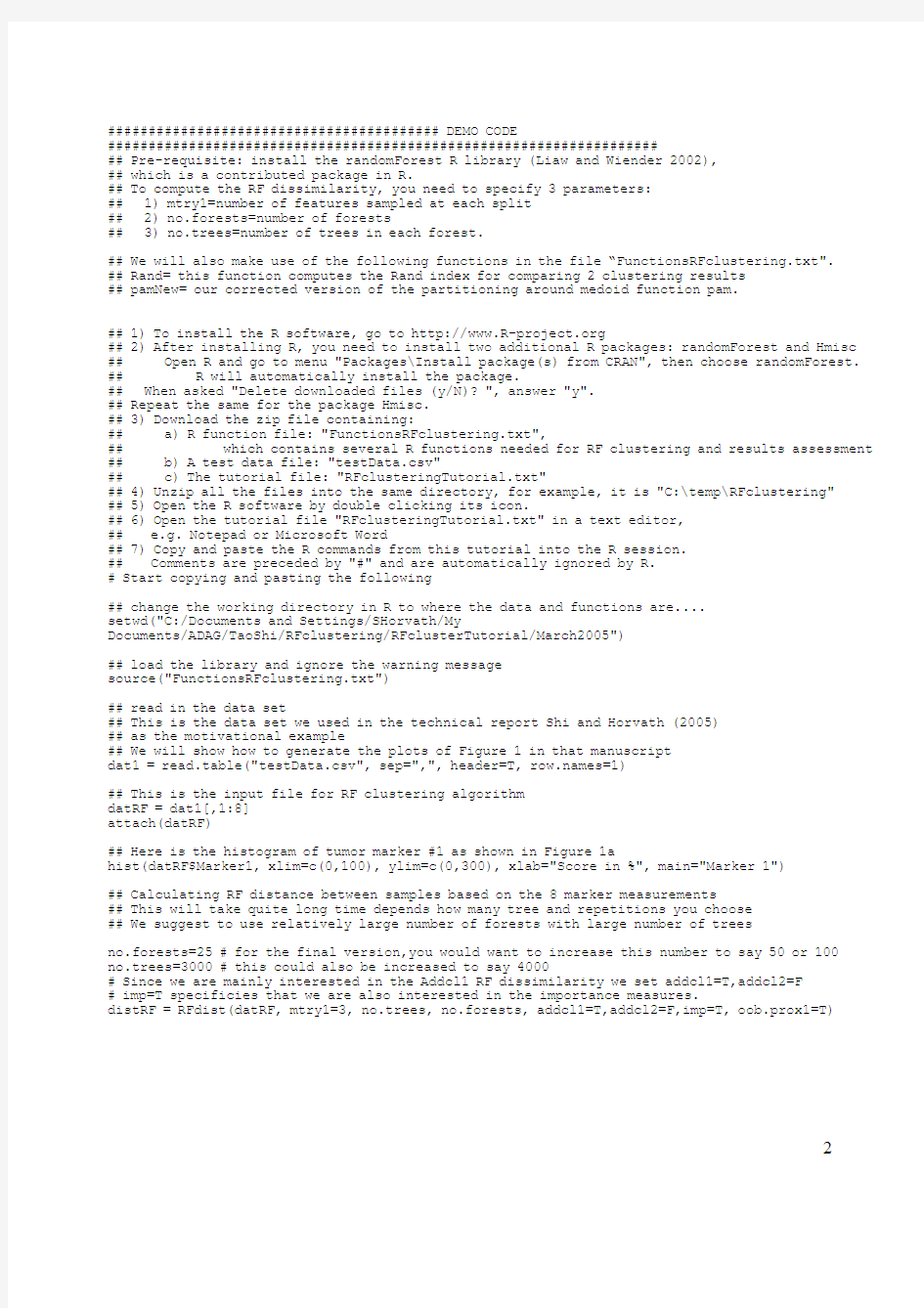
######################################### DEMO CODE

####################################################################

## Pre-requisite: install the randomForest R library (Liaw and Wiender 2002),

## which is a contributed package in R.

## To compute the RF dissimilarity, you need to specify 3 parameters:

## 1) mtry1=number of features sampled at each split

## 2) no.forests=number of forests

## 3) no.trees=number of trees in each forest.

## We will also make use of the following functions in the file “FunctionsRFclustering.txt".

## Rand= this function computes the Rand index for comparing 2 clustering results

## pamNew= our corrected version of the partitioning around medoid function pam.

## 1) To install the R software, go to https://www.sodocs.net/doc/2a7960277.html,

## 2) After installing R, you need to install two additional R packages: randomForest and Hmisc ## Open R and go to menu "Packages\Install package(s) from CRAN", then choose randomForest. ## R will automatically install the package.

## When asked "Delete downloaded files (y/N)? ", answer "y".

## Repeat the same for the package Hmisc.

## 3) Download the zip file containing:

## a) R function file: "FunctionsRFclustering.txt",

## which contains several R functions needed for RF clustering and results assessment ## b) A test data file: "testData.csv"

## c) The tutorial file: "RFclusteringTutorial.txt"

## 4) Unzip all the files into the same directory, for example, it is "C:\temp\RFclustering"

## 5) Open the R software by double clicking its icon.

## 6) Open the tutorial file "RFclusteringTutorial.txt" in a text editor,

## e.g. Notepad or Microsoft Word

## 7) Copy and paste the R commands from this tutorial into the R session.

## Comments are preceded by "#" and are automatically ignored by R.

# Start copying and pasting the following

## change the working directory in R to where the data and functions are....

setwd("C:/Documents and Settings/SHorvath/My

Documents/ADAG/TaoShi/RFclustering/RFclusterTutorial/March2005")

## load the library and ignore the warning message

source("FunctionsRFclustering.txt")

## read in the data set

## This is the data set we used in the technical report Shi and Horvath (2005)

## as the motivational example

## We will show how to generate the plots of Figure 1 in that manuscript

dat1 = read.table("testData.csv", sep=",", header=T, https://www.sodocs.net/doc/2a7960277.html,s=1)

## This is the input file for RF clustering algorithm

datRF = dat1[,1:8]

attach(datRF)

## Here is the histogram of tumor marker #1 as shown in Figure 1a

hist(datRF$Marker1, xlim=c(0,100), ylim=c(0,300), xlab="Score in %", main="Marker 1")

## Calculating RF distance between samples based on the 8 marker measurements

## This will take quite long time depends how many tree and repetitions you choose

## We suggest to use relatively large number of forests with large number of trees

no.forests=25 # for the final version,you would want to increase this number to say 50 or 100 no.trees=3000 # this could also be increased to say 4000

# Since we are mainly interested in the Addcl1 RF dissimilarity we set addcl1=T,addcl2=F

# imp=T specificies that we are also interested in the importance measures.

distRF = RFdist(datRF, mtry1=3, no.trees, no.forests, addcl1=T,addcl2=F,imp=T, oob.prox1=T)

## PAM clustering based on the Addcl1 RF dissimilarity no.clusters = 2

labelRF = pamNew(distRF$cl1, no.clusters)

## PAM clustering based on Euclidean distance labelEuclid = pamNew(dist(datRF), no.clusters)

## Due to the randomness of RF procedure, the exact distance measure will vary a bit ## Therefore, we also include our RF clustering result in our data

##If you want to see our result, you may need to add the following statement #labelRF = dat1$labelRF

## Check the agreement between RF cluster and Euclidean distance cluster fisher.test(table(labelRF, labelEuclid)) ## Fisher’s exact p value

Selected Output

Fisher's Exact Test for Count Data data: table(labelRF, labelEuclid) p-value = 1.216e-15

## Define a new clustering label based on labelRF and labelEuclid ## labelNew=1, if labelRF=1 and labelEuclid=1 ## labelNew=2, if labelRF=1 and labelEuclid=2 ## labelNew=3, if labelRF=2 and labelEuclid=1 ## labelNew=4, if labelRF=2 and labelEuclid=2 labelNew = ifelse(labelRF==1&labelEuclid==1, 1, ifelse(labelRF==1&labelEuclid==2, 2,

ifelse(labelRF==2&labelEuclid==1, 3, 4)))

## check survival difference as in Figure 1b

## variables "time" and "event" in dat1 are survival time and cencering indicator, respectively

## NOTE: the RF clusters are more meaningful with respect to survival time. fit1 = survfit(Surv(time, event)~labelNew, data=dat1, conf.type="log-log")

mylegend=c("RF cluster 1, Euclid cluster 1", "RF cluster 1, Euclid cluster 2", "RF cluster 2, Euclid cluster 1","RF cluster 2, Euclid cluster 2") plot(fit1, conf.int=F,col= unique(labelNew), lty=1:4, xlab="Time to death ",ylab="Survival",legend.text=mylegend, lwd=1,mark.time=TRUE)

#Output: Kaplan Meier plot: Proportion of Surviving Patients versus Time

246

81012

0.00.20.40.6

0.8

1.0

Time to death (years)

S u r v i v a l

RF cluster 1, Euclid cluster 1RF cluster 1, Euclid cluster 2RF cluster 2, Euclid cluster 1RF cluster 2, Euclid cluster 2

## Figure 1c (need library 'sma')

library(sma)

colorh = labelNew

order1 = order(labelNew)

par(mfrow=c(1,1))

plot.mat( scale(datRF[order1,]), rlabels=colorh[order1], rcols=colorh[order1],

clabels=dimnames(datRF)[[2]], ccols=1, margin=0.5)

# Heatmap plot: rows correspond to observations (tumor samples) columns to tumor markers

# the rows are sorted according to the color label defined by the K-M plot above

# Messages:

# In the green and blue samples (i.e. RF cluster 2) markers 1 and 2 are under-expressed (green) # while in red and blue samples, marker 4 is over-expressed (red)

## Using rpart tree the dissect the relationship between RF clusters and markers expression value ## need library 'rpart' library(rpart)

rp1 = rpart(factor(labelRF)~., datRF)

plot(rp1); text(rp1, all=T, use.n=T, cex=0.7)

|Marker1>=67.5

Marker3< 16.04

Marker2>=81.67

Marker4< 22.5

1248/59

1241/27

1222/8

1217/2

25/6

119/19

12

27/32

summary(rp1)

Selected Output Call:

rpart(formula = factor(labelRF) ~ ., data = datRF) n= 307

CP nsplit rel error xerror xstd 1 0.42372881 0 1.0000000 1.0000000 0.11701207 2 0.12711864 1 0.5762712 0.6610169 0.09889595 3 0.01694915 3 0.3220339 0.4406780 0.08268346 4 0.01000000 4 0.3050847 0.4745763 0.08549878

Node number 1: 307 observations, complexity param=0.4237288 predicted class=1 expected loss=0.1921824 class counts: 248 59 probabilities: 0.808 0.192

left son=2 (268 obs) right son=3 (39 obs) Primary splits:

Marker1 < 67.5 to the right, improve=35.27559, (0 missing) Marker2 < 92.5 to the right, improve=30.47311, (0 missing) Marker3 < 16.04165 to the left, improve=27.02816, (0 missing) Marker4 < 23.33335 to the left, improve=22.40886, (0 missing) Marker5 < 41.66665 to the left, improve=13.10948, (0 missing) Surrogate splits:

Marker2 < 30.5952 to the right, agree=0.906, adj=0.256, (0 split) Marker3 < 31.25 to the left, agree=0.883, adj=0.077, (0 split)

Node number 2: 268 observations, complexity param=0.1271186 predicted class=1 expected loss=0.1007463 class counts: 241 27 probabilities: 0.899 0.101

left son=4 (230 obs) right son=5 (38 obs) Primary splits:

Marker3 < 16.04165 to the left, improve=14.116220, (0 missing) Marker2 < 81.66665 to the right, improve=10.177620, (0 missing) Marker5 < 39.58335 to the left, improve=10.158150, (0 missing) Marker4 < 23.33335 to the left, improve= 9.135023, (0 missing) Marker8 < 94.14285 to the left, improve= 3.628743, (0 missing) Surrogate splits:

Marker2 < 43.125 to the right, agree=0.866, adj=0.053, (0 split) Marker5 < 55 to the left, agree=0.866, adj=0.053, (0 split) ETC

## This suggests to construct a rule based on first two splits

rule1 = 2-I(datRF$Marker1>=67.5 & datRF$Marker3<16.04) table(rule1,labelRF) # 11.4 percent disagreement labelRF

rule1 1 2 1 222 8 2 26 51

## Another rule using the sencond highest ranking split for the split number 2 (Marker2>=81.67) ## leads to better agreement between the rule and RF clusters rule1 = 2.0-I(datRF$Marker1>=67.5 & datRF$Marker2>=81.67) table(rule1,labelRF) # 9.4 percent disagreement

labelRF rule1 1 2 1 222 8 2 26 51

## This means that we can only use two markers to explain the RF clusters (Figure 1d)

plot(jitter(Marker1,5),jitter(Marker2,5), col=labelNew, cex=1.5, xlab="Marker 1", ylab="Marker 2") abline(h=81.67); abline(v=67.5)

2040

6080100

20406080100

Marker 1

M a r k e r

2

################################################################################################## ##################################Simulated Example #######################################

## The following codes show how to arrive at the plots for our simulation example 'ExRule'.

## Here is how we simulate the data for the example 'ExRule'

## There are 2 signal variables.

## For observations in cluster 1 and cluster 2, the 2 signal variables X1 and X2 have random

## uniform distributions on the intervals U[0.8, 1] and U[0, 0.8], respectively.

## Thus cluster 1 observations can be predicted using the

## threshold rule X1 > 0.8 and X2 > 0.8.

## We simulate 150 cluster 1 observations and 150 cluster 2 observations.

## Noise variable X3 is simulated to follow a binary (Bernoulli) distribution with hit probability ## =0.5, which is independent of all other variables.

## Noise variables X4, ... ,X10 are simulated by randomly permuting variable X1,

## i.e. they follow the same distribution of X1 but are independent of all other variables.

nobs = 300

ratio1 = 0.5

X1 = c(runif(nobs*ratio1, min=0.8, max=1), runif((1-ratio1)*nobs,min=0,max=0.8) )

X2 = c(runif(nobs*ratio1, min=0.8, max=1), runif((1-ratio1)*nobs,min=0,max=0.8) )

X3 = sample(rep(c(0,1),c(nobs/2,nobs/2) ))

data1 =

data.frame(X1,X2,X3=X3,X4=sample(X1),X5=sample(X1),X6=sample(X1),X7=sample(X1),X8=sample(X1),X9=sa mple(X1),X10=sample(X1))

## Generate RF dissimilarity

distRF2 = RFdist(data1, mtry1=3, 1000, 7, addcl1=T,addcl2=T,imp=T, oob.prox1=T)

## Classical Multidimensional scaling based on RF or Euclidean distances

cmd1 = cmdscale(as.dist(distRF2$cl1),2)

cmd2 = cmdscale(as.dist(distRF2$cl2),2)

cmdEuclid = cmdscale(dist(data1),2)

## Isotonic Multidimensional scaling based on RF or Euclidean distances

iso1 = isoMDS(as.dist(distRF2$cl1),k=2)$points

iso2 = isoMDS(as.dist(distRF2$cl2),k=2)$points

isoEuclid = isoMDS(dist(data1),k=2)$points

## Color the points based on X1 and X3

color1 = ifelse( X1>=0.8 & X3==0, "black",

ifelse( X1>=0.8 & X3==1, "red",

ifelse( X1<0.8 & X3==1, "blue","green")))

## Figure 3

par(mfrow=c(3,3))

plot(cmd1,col=color1,xlab=NA, ylab=NA, main="Addcl1, cMDS" ) plot(iso1,col=color1,xlab=NA, ylab=NA, main="Addcl1, isoMDS")

plot(distRF2$imp1[,4] ,xlab="variables",ylab="Gini Index Measure", main="Addcl1, Variable Imp.") plot(cmd2,col=color1,xlab=NA, ylab=NA, main="Addcl2, cMDS") plot(iso2,col=color1,xlab=NA, ylab=NA,main="Addcl2, isoMDS")

plot(distRF2$imp2[,4] ,xlab="variables",ylab="Gini Index Measure", main=" Addcl1, Variable Imp.") plot(cmdEuclid,col=color1,xlab=NA, ylab=NA, main="Euclidean, cMDS" ) plot(isoEuclid,col=color1,xlab=NA, ylab=NA, main="Euclidean, isoMDS")

plot(apply(data1,2,var) ,xlab="variables",ylab="Variance", main="Variable Variance")

-0.15-0.050.050.15

-0.2

0.1

Addcl1, cMDS

-0.2

-0.10.00.10.2

-0.2

0.1

Addcl1, isoMDS 246810

1030

Addcl1, Variable Imp.

variables

G i n i I n d e x M e a s u r e

-0.3-0.2-0.1

0.00.10.2-0.2

0.1

Addcl2, cMDS

-0.4-0.20.00.20.4-0

.100.10

Addcl2, isoMDS 246810

50

150 Addcl1, Variable Imp.

variables

G i n i I n d e x M e a s u r e

-0.6-0.20.00.20.40.6-0.5

1.0

Euclidean, cMDS

-1.0-0.50.00.5

1.0

-0.5

1.0

Euclidean, isoMDS

246810

0.10

0.25

Variable Variance

variables

V a r i a n c e

#THE END