Anisotropic Electron-Phonon Coupling Uncovered By Angle-Resolved Photoemission

a r X i v :c o n d -m a t /0409426v 1 [c o n d -m a t .s u p r -c o n ] 16 S e p 2004

Anisotropic Electron-Phonon Coupling Uncovered By

Angle-Resolved Photoemission

T.P.Devereaux,a ,?T.Cuk,b Z.-X.Shen,b and N.Nagaosa c

a

Department of Physics,University of Waterloo,Waterloo,Ontario,N2L 3G1,Canada

b

Dept.of Physics,Applied Physics and Stanford Synchrotron Radiation Laboratory,Stanford University,California 94305,USA

c

Department of Applied Physics,University of Tokyo,Bunkyo-ku,Tokyo 113-8656,Japan

The physics underlying the peculiar behavior of the high temperature superconductors in the normal state and the high transition temperatures themselves is far from understood.While the importance of magnetic interactions has been widely pointed out,a number of experimental ?ndings strongly suggest that electron-phonon coupling must play a role in these materials.These ?ndings include strong phonon renormalizations with temperature and/or doping seen in neutron and Raman scattering[1,2],the doping dependence of the isotope e?ect of the transition temperature[3],the iso-tope dependence of the super?uid density[4],and lastly the pressure,layer and material dependence of T c it-self.

In this paper we focus attention on some recent de-velopments coming from angle-resolved photoemission (ARPES)experiments and theoretical developments of anisotropic electron-phonon interactions in general.Initially,the attention to bosonic renormaliza-tion e?ects in cuprate superconductors was focussed on a “kink”in the electronic dispersion near 50-70meV for nodal electrons[5,6,7,8,9]or solely below

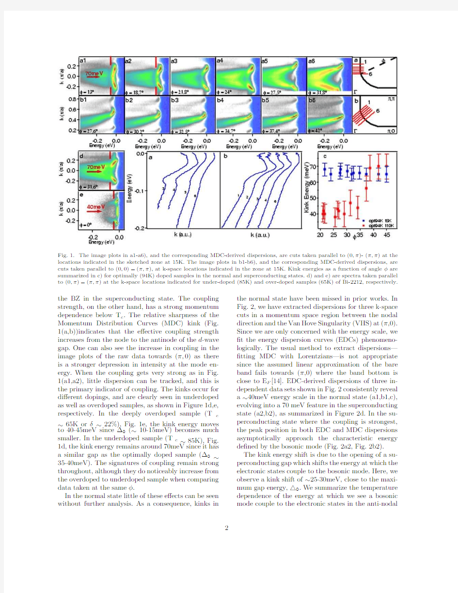
Fig.1.The image plots in a1-a6),and the corresponding MDC-derived dispersions,are cuts taken parallel to(0,π)-(π,π)at the locations indicated in the sketched zone at15K.The image plots in b1-b6),and the corresponding MDC-derived dispersions,are cuts taken parallel to(0,0)?(π,π),at k-space locations indicated in the zone at15K.Kink energies as a function of angleφare summarized in c)for optimally(94K)doped samples in the normal and superconducting states.d)and e)are spectra taken parallel to(0,π)?(π,π)at the k-space locations indicated for under-doped(85K)and over-doped samples(65K)of Bi-2212,respectively.

the BZ in the superconducting state.The coupling

strength,on the other hand,has a strong momentum dependence below T c.The relative sharpness of the

Momentum Distribution Curves(MDC)kink(Fig.

1(a,b))indicates that the e?ective coupling strength increases from the node to the antinode of the d-wave

gap.One can also see the increase in coupling in the

image plots of the raw data towards(π,0)as there is a stronger depression in intensity at the mode en-

ergy.When the coupling gets very strong as in Fig.

1(a1,a2),little dispersion can be tracked,and this is the primary indicator of coupling.The kinks occur for

di?erent dopings,and are clearly seen in underdoped

as well as overdoped samples,as shown in Figure1d,e, respectively.In the deeply overdoped sample(T c

～65K orδ～22%),Fig.1e,the kink energy moves to40-45meV since?0(～10-15meV)becomes much smaller.In the underdoped sample(T c～85K),Fig. 1d,the kink energy remains around70meV since it has

a similar gap as the optimally doped sample(?0～35-40meV).The signatures of coupling remain strong throughout,although they do noticeably increase from the overdoped to underdoped sample when comparing data taken at the sameφ.

In the normal state little of these e?ects can be seen

without further analysis.As a consequence,kinks in the normal state have been missed in prior works.In Fig.2,we have extracted dispersions for three k-space cuts in a momentum space region between the nodal direction and the Van Hove Singularity(VHS)at(π,0). Since we are only concerned with the energy scale,we ?t the energy dispersion curves(EDCs)phenomeno-logically.The usual method to extract dispersions—?tting MDC with Lorentzians—is not appropriate since the assumed linear approximation of the bare band fails towards(π,0)where the band bottom is close to E F[14].EDC-derived dispersions of three in-dependent data sets shown in Fig.2consistently reveal a～40meV energy scale in the normal state(a1,b1,c), evolving into a70meV feature in the superconducting state(a2,b2),as summarized in Figure2d.In the su-perconducting state where the coupling is strongest, the peak position in both EDC and MDC dispersions asymptotically approach the characteristic energy de?ned by the bosonic mode(Fig.2a2,Fig.2b2). The kink energy shift is due to the opening of a su-perconducting gap which shifts the energy at which the electronic states couple to the bosonic mode.Here,we observe a kink shift of～25-30meV,close to the maxi-mum gap energy,△0.We summarize the temperature dependence of the energy at which we see a bosonic mode couple to the electronic states in the anti-nodal

k (π/a)k (π/a)φFig.2.EDC(a1,b1,c)derived dispersions in the normal state (107K and115K).φand the cut-direction are noted in the insets.The red dots are the data;the?t to the curve(dashes, black)below the40meV line is a guide to the eye.a2)and b2) are MDC derived dispersions at the same location and direction as in a1)and b1),but in the superconducting state(15K).In a2)and b2)we also plot the peak(I)and hump positions(II)of the EDCs for comparison.The inset of a2)shows the expected behavior of a Bogoliubov type gap opening.The s-like shape below the gap energy is an artifact of how the MDC handles the back-bend of the Bogoliubov quasiparticle.d)kink positions as a function ofφin the anti-nodal region.

region in Figs.1(c)and2(d):the kink energies are at ～40meV above T c near the anti-nodal region and in-crease to～70meV below T c.Because the band mini-mum is too close to E F,the normal state～40meV kink cannot easily be seen belowφ～20o.

By comparing the di?erent cut directions,one can clearly see that the coupling is extended in the Bril-louin zone and has a similar energy scale throughout, near～70meV.Moreover,the signatures of coupling increase signi?cantly toward(π,0)or smallerφ.The clear minimum in spectral weight seen near70meV in Fig.2a1)and2a2)indicates strong mixing of the elec-tronic states with the bosonic mode where the two bare dispersions coincide in energy.

The above described experimental observations are di?cult to reconcile in the spin resonance mode sce-nario.The kink is clearly observed at40meV in the normal state at optimal doping while the41meV spin resonance mode exists only below T c[15].The kink is sharp in the superconducting state of a deeply over-doped Bi2212sample(Fig.1e,consistent with data of [12])while no spin resonance mode has been reported, or is expected to exist at this doping.In addition the kink seen in under-doped Bi2212(Fig.1d)is just as sharp as in the optimally doped case,while the neutron resonance peak is much broader[15].Lastly,it is di?-cult to account for the strong kink e?ect seen through-out the BZ from the spin mode since the mode’s spec-tral weight is only2%[16]as it may only cause a strong enough kink e?ect if the interaction with electrons is highly concentrated in k-space[17].

On the other hand,it has been argued that the bosonic renormalization e?ect may be reinterpreted as a result of a coupling to the half-breathing in-plane Cu-O bond-stretching phonon for nodal directions[6,7]and the out-of-plane out-of-phase O buckling B1g phonon for anti-nodal directions[13].This re-interpretation has the clear advantage over the spin resonance in that it naturally explains why the band renormalization e?ect is observed under three circumstances:1)in materials where no spin mode has been detected,2)in the nor-mal state,and3)in the deeply overdoped region where the spin mode is neither expected nor observed.How-ever this interpretation also requires that the electron-phonon interaction be highly anisotropic and its im-pact on the electrons be strongly enhanced in the su-perconducting state.This is something one does not expect a priori.

We now show that the anisotropy of the electron-phonon interaction of these phonons,when formulated within the same framework as that used to explain phonon lineshape changes observed via Raman and neutron measurements[1,2,18,19],explain the ob-served momentum and temperature dependence of the data,leading to uni?ed understanding of band renormalizations.The electron-phonon interactions are very anisotropic as a consequence of the following four properties of the cuprates:1)the symmetry of the phonon polarizations and electronic orbitals in-volved leading to highly anisotropic electron-phonon coupling matrix elements g(k,q);2)the kinematic constraint related to the anisotropy of the electronic band structure and the van Hove singularity(VHS);

3)the d-wave superconducting gap,and4)the near degeneracy of energy scales of the B1g phonon,the superconducting gap,and the VHS.

We consider a tight-binding three-band Hamiltonian modi?ed by B1g buckling vibrations as considered in Ref.[18]and in-plane breathing vibrations as consid-ered in Ref.[20]:

H= n,σ?Cu b?n,σb n,σ

+ n,δ,σ{?O+eE z u Oδ(n)}a?n,δ,σa n,δ,σ

+ n,δ,σPδ[t?Qδg dp u Oδ(n)](b?n,σa n,δ,σ+h.c.) +t′ n,δ,δ′P′δ,δ′(a?n,δa n,δ′,σ+h.c)(1) with Cu-O hopping amplitude t,O-O amplitude t′,and

Fig.3.Plots of the electron-phonon coupling|g(k,q)|2for initial k and scattered k′=k?q states on the Fermi sur-face for the buckling mode(left panels)and breathing mode (right panels)for initial fermion k at an anti-nodal(top pan-els)and nodal(bottom panels)point on the Fermi surface, as indicated by the arrows.The red/blue color indicates the maximum/minimum of the el-ph coupling vertex in the BZ for each phonon.

?d,p denoting the Cu and O site energies,respectively.

Here aα=x,y,a?α=x,y(b,b?)annihilates,creates an elec-tron in the Oα(Cu)orbital,respectively.The overlap factors Qδ,Pδ,and P′δ,δ′are given in our notation as Q±x=Q±y=±1;P±x=?P±y=±1;P′±x,±y=1=?P′?x,±y.For the half-breathing mode we consider only couplings g dp=q0t(with1/q0a length scale)arising

from modulation of the covalent hopping amplitude

t[20,21].For the B1g mode a coupling to linear order in the atomic displacements arises from a local c-axis oriented crystal?eld E z which breaks the mirror plane symmetry of the Cu-O plane[18].Such a?eld may be due to static buckling or di?erent valences of ions on either side of the Cu-O plane,orthorhombic tilts of the octahedra,or may be generated dynamically.

The amplitudesφof the tight-binding wavefunctions

forming the anti-bonding band with energy dispersion

?(k)arising from Eq.1include the symmetry of the p,d wavefunctions of the Cu-O plane.The speci?c trans-formation is constructed from the projected part of

the tight-binding wavefunctions b k

,σ=φb(k)d k

,σ

and

aα,k,σ=φα(k)d k

,σ

,

φb(k)=

1

N(k)

[?(k)t x,y(k)?t′(k)t y,x(k)],(3)

with N2(k)=[?2(k)?t′2(k)]2+[?(k)t x(k)?t′(k)t y(k)]2+[?(k)t y(k)?t′(k)t x(k)]2,tα(k)= 2t sin(kαa/2),and t′(k)=4t′sin(k x a/2)sin(k y a/2). In particular if k resides on the Fermi surface,then

φF S b (k)=?|t′(k)|

t′(k)2+t x(k)2+t y(k)2

,(4)

φF S

x,y

(k)=±isgn[t′(k)]t y,x(k)

t′(k)2+t x(k)2+t y(k)2

.

(5)

Fig.4.Plots of the electron-phonon couplingλk in the?rst

quadrant of the BZ for the buckling mode(right top panel)

and breathing mode(right bottom panel).The color scale is

shown on the right for each phonon.The left panel shows

energy contours for the band structure used[23].

The full anisotropy of the electron-phonon cou-

pling comes from the projected wavefunctions in

combination with the phonon eigenvectors:H el?ph=

1

N k,q,σ,μgμ(k,q)c?k,σc k+q,σ[a?μ,q+aμ,?q].Ne-

glecting the motion of the heavier Cu atoms compared

to O in the phonon eigenvectors the form of the re-

spective couplings can be compactly written as

g B

1g

(k,q)=eE z 4M O M(q)?B1g(6)

× φx(k)φx(k′)cos(q y a/2)?φy(k)φy(k′)cos(q x a/2)

g br(k,q)=g dp 2M O?br α=x,y(7)

× φb(k′)φα(k)cos(k′αa/2)?φb(k)φα(k′)cos(kαa/2) ,

with M(q)=[cos2(q x a/2)+cos2(q y a/2)]/2and

k′=k-q.Here we have neglected an overall irrele-

vant phase factor.The anisotropy can be shown at

small momentum transfers q where g B

1g

(k,q=0)～

cos(k x a)?cos(k y a),while g br～sin(qa)for any k.

Also for large momentum transfer q=(π/a,π/a),

g B

1g

vanishes for all k while g br has its maximum for

k located on the nodal points of the Fermi surface.

While this q-dependence has been the focus before in

context with a d x2?y2pairing mechanism[22],the de-

pendence on fermionic wavevector k has usually been

overlooked.This strong momentum dependence of the

B1g coupling implies that resistivity measurements

would be sensitive only to the weaker part of the

electron-phonon coupling,in agreement with experi-

ments.It is exactly this fermionic dependence which

we feel is crucially needed to interpret ARPES data.

Fig3plots|g(k,q)|2as a function of phonon

scattered momentum q connecting initial k and?nal

Fig.5.Image plots of the calculated spectral functions in the normal(a1,b1,c1)and superconducting(a2,b2,c2)states compared to the spectral functions in the normal(a3,b3,c3)and superconducting(a4,b4,c4)states measured in Bi2Sr2Ca0.92Y0.08Cu2O8+δ(Bi-2212)[13]for momentum cuts a,b,c shown in the right-most panel and in Figure 2.The same color scale is used for the normal/superconducting pairs within each cut,but the scaling for the data and the calculation are separate.The red markers indicate70meV in the superconducting state.

k′=k?q fermion states both on the Fermi surface. Here we have adopted a?ve-parameter?t to the band

structure?(k)used previously for optimally doped Bi-

2212[23].For an anti-nodal initial fermion k AN,the coupling to the B1g phonon is largest for q=0and2k F

scattering to an anti-nodal?nal state.The coupling to

the breathing mode is much weaker overall,and is espe-cially weak for small q and mostly connects to fermion

?nal states at larger q.For a nodal fermion initial state

k N,the B1g coupling is suppressed for small q and has a weak maximum towards anti-nodal?nal states,while

the breathing mode attains its largest value for scat-

tering to other nodal states,particularly to state?k N. In Fig.4we plotλk for each k point in the BZ in the

normal state,where we have de?ned[24]:

λk=

2

N kδ(?(k))the density of states per spin at the Fermi level.As a result of the anisotropy of the

coupling constant,large enhancements of the coupling near the anti-node for the B1g phonon,and nodal di-rections for the breathing phonon mode are observed, respectively,which are an order of magnitude larger thanλ=1

2eE z as a representative value for the cou-pling to the breathing mode.These values lead to net couplings similar to that obtained from LDA calcula-tions for an in?nite layer compound CaCuO2which develops a static dimple[24].

The Nambu-Eliashberg electron-phonon self-energy determines bosonic features in the spectral function[25]:?Σ(k,iωm)=iωm(1?Z(k,iωm))?τ0+χ(k,iωm)?τ3+Φ(k,iωm)?τ1with

?Σ(k,iω

m

)=

1

(iωm)2?E2(p)

and E2(k)=?2(k)+?2(k),with?τi=0···3are Pauli matrices.We take?(k)=?0[cos(k x a)?cos(k y a)]/2with?0= 35meV.The bare phonon propagators are taken as

D0μ(q,i?ν)=1

i?ν??μ

?1

π

ImG11(k,iω→ω+iδ)is determined from Eq.9with?G(k,iωm)= [?τ0iωm Z(k,iωm)?(?(k)+χ(k,iωm))?τ3?Φ(k,iωm)?τ1]?1 and the coupling constants given by Eq.6-7.Here we consider three di?erent cuts as indicated in Fig.4: along the nodal direction(k x=k y,denoted by c), and two cuts parallel to the BZ face(k y=0.75π/a, b)and(k y=0.64π/a,a)where bilayer e?ects are not severe[13].

Our results for the three cut directions are shown in Fig5for the normal(T=110K)and supercon-ducting(T=10K)states.Very weak kink features are seen in the normal state,with a smeared onset of broadening at the phonon energy due to the measure-ment temperature.A much more pronounced kink at 70meV in the superconducting state is observed for all the cuts along with a sharp onset of broadening,in excellent agreement with the data[13],shown also in Fig.5.In the superconducting state,the kink sharp-ens due to the singularity in the superconducting den-sity of states from the anti-nodal regions.Thus cut a exhibits the strongest signatures of coupling,showing

an Einstein like break up into a band that follows the phonon dispersion,and one that follows the electronic one.In cut b,a weaker signature of coupling manifests itself in an s?like renormalization of the bare band that traces the real part of the phonon self-energy,while in cut c,where the coupling to the B1g phonon is weak-est,the electron-phonon coupling manifests itself as a change in the velocity of the band.The agreement is very good,even for the large change in the electron-phonon coupling seen between cuts a and b,separated by only1/10th of the BZ.

We now discuss the reason for the strong anisotropy as a result of a concurrence of symmetries,band struc-ture,d?wave energy gap,and energy scales in the electron-phonon problem.In the normal state,weak kinks are observed at both phonon frequencies,but more pronounced at70meV for cut c and at36meV for cut a,as expected from the anisotropic couplings shown in Fig.3.However this is also a consequence of the energy scales of the phonon modes and the bottom of electronic band along the cut direction as shown in Fig.4.Further towards the anti-node,another inter-esting e?ect occurs.As one considers cuts closer to the BZ axis,the bottom of the band along the cut rises in energy and the breathing phonon mode lies below the bottom of the band for(k x=0,k y>0.82π/a)and so the kink feature for this mode disappears.This is the usual e?ect of a Fano redistribution of spectral weight when a discrete excitation lies either within or outside of the band continuum[26].This thus can be used to open”windows”to examine the coupling of electrons to discrete modes in general.Taken together,this nat-urally explains why the normal state nodal kink is near 70meV[5,6,7,8,9]while the anti-nodal kink is near40 meV[10,11,12,13].

In the superconducting state the bare band renor-malizes downward in energy due to the opening of the gap and gives the strongest e?ect for the anti-nodal re-gion where the gap is of the order of the saddle point en-ergy.The B1g coupling becomes dramatically enhanced by the opening of the gap at a frequency close to the frequency of the phonon itself,and leads to the dra-matic renormalization of the phonon observed in Ra-man and neutron measurements[1].Yet the breathing coupling does not vary dramatically as the large gap region is not weighted as heavily by the coupling con-stant.As a consequence,the B1g mode dominates and clear kinks in the data are revealed at around70meV -the B1g energy plus the gap.Indeed a much weaker kink at105meV from the breathing phonon shows at higher energies for the nodal cut but this kink becomes weaker away from nodal directions as the coupling and the band bottom along the cut moves below the phonon frequency so that the“energy window”closes. Finally we plot in Fig.6the superconducting density of states(DOS)?1/πImG11(k,ω)calculated with

the Fig.6.Superconducting density of states calculated with the electron-phonon self energy for three di?erent values of the electric?eld eE z=0(black),1.85(blue),and3.2(red),in units of eV/?A,respectively.The yellow dashed lines indicate the energies?B1g+?0and?br+?0.

electron-phonon contributions from both the breath-ing and B1g phonons to the self energy determined via Eq.9for three di?erent values of the B1g coupling con-stant parametrized by the crystal?eld eE z.We have ?xed the relative breathing coupling at q0t=2

√

[1] B.Friedl et al.,Phys.Rev.Lett.65,915(1990);N.Pyka

et al.,Phys.Rev.Lett.70,1457(1993);D.Reznik et al., Phys.Rev.Lett.75,2396(1995).

[2]S.L.Chaplot et al.,Phys.Rev.B52,7230(1995);R.J.

McQueeney et al.,Phys.Rev.Lett.82,628(1999);87, 077001(2001);J.-H.Chung et al.,Phys.Rev.B67,014517 (2003);S.Sugai et al.,Phys.Rev.B68,184504(2003).

[3]J.P.Franck,in Physical Properties of High Tc

Superconductors IV,edited by D.M.Ginsberg(World Scienti?c,Singapore,1994),p.189;M.K.Crawford,M.N.

Kunchur,W.E.Farneth,E.M.McCarron,and S.J.Poon, Phys.Rev.B41,282(1990).

[4]R.Khasanov et al,Phys.Rev.Lett.92057602(2004);

cond-mat/0404428.

[5]P.V.Bogdanov et al.,Phys.Rev.Lett.85,2581(2000).

[6] https://www.sodocs.net/doc/448821628.html,nzara et al.,Nature412,510(2001).

[7]X.J.Zhou et al.Nature423,398(2003).

[8] A.Kaminski et al.,Phys.Rev.Lett86,1070(2001).

[9]P.D.Johnson et al.,Phys.Rev.Lett87,177007(2001).

[10]T.K.Kim et al.,Phys.Rev.Lett.91,167002(2003).

[11]T.Sato et al.,Phys.Rev.Lett91,157003(2003).

[12]A.D.Gromko et al.,Phys.Rev.B,68,174520(2003).

[13]T.Cuk et al.,Phys.Rev.Lett.93,117003(2004).

[14]https://www.sodocs.net/doc/448821628.html,Shell,E.Jensen,T.Balasubramanian Phys.Rev.B

61,2371(2000).

[15]H.F.Fong Phys.Rev.Lett.75,316(1995);P.Dai et al.,

Phys.Rev.B63,054525(2001).

[16]H.-Y.Kee,S.A.Kivelson,G.Aeppli,Phys.Rev.Lett.88,

257002(2002).

[17]A.Abanov et al.,Phys.Rev.Lett.89,177002(2002).

[18]M.Opel et al.,Phys.Rev.B60,9836(1999);T.P.

Devereaux,A.Virosztek,and A.Zawadowski Phys.Rev.

B59,14618(1999);51,505(1995).

[19]T.P.Devereaux et al.,Phys.Rev.Lett.93,117004(2004).

[20]S.Bari?s i′c,Phys.Rev.B5,932(1972).

[21]The coupling g d arising from modulation of Cu site

energies leads to a coupling which only depends on momentum transfers on not on fermion momentum[20].

[22]D.J.Scalapino,J.Phys.Chem.Solids56,1669(1995);A.

Nazarenko and E.Dagotto,Phys.Rev.B53,2987(1996);

O.Jepsen et al.,J.Phys.Chem.Solids59,1718(1998);

T.S.Nunner,J.Schmalian and K.H.Bennemann,Phys.

Rev.B59,8859(1999).

[23]M.R.Norman et al.,Phys.Rev.B64,184508(2001).

M.Eschrig and M.R.Norman,Phys.Rev.Lett.85,3261 (2000);Phys.Rev.B67,144503(2003);A.V.Chubukov and M.R.Norman,cond-mat/0402304.cond-mat/0403766 [24]O.Jepsen et al.,J.Phys.Chem.Solids59,1718(1998);

O.K.Andersen et al.,J.of Low Temp.Phys.105,285 (1996);S.Y.Savrasov and O.K.Andersen,Phys.Rev.

Lett.77,4420(1996).

[25]A.W.Sandvik,D.J.Scalapino,N.E.Bickers,Phys.Rev.

B69,094523(2004).

[26]U.Fano,Phys.Rev.124,1866(1961).

[27]E.W.Hudson,S.H.Pan,A.K.Gupta,K.-W.Ng,and J.C.

Davis,Science285,88(1999);J.F.Zasadzinski,L.Co?ey, P.Romano,and Z.Yusof,Phys.Rev.B68,180504(2003).

用Abaqus进行压电(Piezoelectric)悬臂梁模拟入门详解_第二版

用ABAQUS 进行压电（Piezoelectric ）悬臂梁模拟入门详解 作者：X.C. Li 2014.8 （第二版） 本文着重讲述在用ABAQUS 模拟压电材料时，材料常数的设置。希望对入门者有所帮助。如果发现错误请发邮件到：Lxc1975@https://www.sodocs.net/doc/448821628.html, 。 1. 问题描述 柱状体10×4×2如下图 左端固定，右端自由；上表面受均匀压力500；上、下表面电压分别为50V 、0V 。 压电材料PZT-4，选z-方向（该方向上尺寸为2）为极化方向，文献Haojiang Ding, Jian Liang ： The fundamental solutions for transversely isotropic piezoelectricity and boundary element method 给出的材料常数 111213334466111212.6, 7.78, 7.43, 11.5, 2.56, 0.5()c c c c c c c c ======-（10210N m -??）； 15313312.7, 5.2, 15.1 e e e ==-=（-2C m ?）； -121103300=730, =635, =8.8541910 λελεε???（1-1C V m -?） 这些常数在ABAQUS 中的输入将在本文2.3中详细说明。必须说明的是以上材料常数所对应的的本构关系： 111213121113131333444466 0 0 0 0 0 0 0 0 00 0 0 0 00 0 0 0 00 0 0 0 0 xx xx yy yy zz zz yz yz zx xy c c c c c c c c c c c c σεσεσεσγσγσ??????????????????=??????????????????? ???31313315150 0 0 0 0 0 0 0 0 00 0 0x y z zx xy e e E e E e E e γ??????????????????????-???????????????????????????? 15111511333131330 0 0 0 0 0 00 0 0 0 00 00 0 0 0 0xx yy x x zz y y yz z z zx xy E D e D E e e e e D E εελελγλγγ??????????????????????????=+??????????????????????????????????

An anisotropic Phong BRDF model

An Anisotropic Phong BRDF Model Michael Ashikhmin Peter Shirley August13,2000 Abstract We present a BRDF model that combines several advantages of the various empirical models cur-rently in use.In particular,it has intuitive parameters,is anisotropic,conserves energy,is reciprocal,has an appropriate non-Lambertian diffuse term,and is well-suited for use in Monte Carlo renderers. 1Introduction Physically-based rendering systems describe re?ection behavior using the bidirectional re?ectance distri-bution function(BRDF).For a detailed discussion of the BRDF and its use in computer graphics see the volumes by Glassner[2].At a given point on a surface the BRDF is a function of two directions,one toward the light and one toward the viewer.The characteristics of the BRDF will determine what“type”of material the viewer thinks the displayed object is composed of,so the choice of BRDF model and its parameters is important.We present a new BRDF model that is motivated by practical issues.A full rationalization for the model and comparison with previous models is provided in a seperate technical report[1]. The BRDF model described in the paper is inspired by the models of Ward[8],Schlick[6],and Neimann and Neumann[5].However,it has several desirable properties not previously captured by a single model. In particular,it 1.obeys energy conservation and reciprocity laws, 2.allows anisotropic re?ection,giving the streaky appearance seen on brushed metals, 3.is controlled by intuitive parameters, 4.accounts for Fresnel behavior,where specularity increases as the incident angle goes down, 5.has a non-constant diffuse term,so the diffuse component decreases as the incident angle goes down, 6.is well-suited to Monte Carlo methods. The model is a classical sum of a“diffuse”term and a“specular”term. ρ(k1,k2)=ρs(k1,k2)+ρd(k1,k2).(1) For metals,the diffuse componentρd is set to zero.For“polished”surfaces,such as smooth plastics,there is both a diffuse and specular appearance and neither term is zero.For purely diffuse surfaces,either the traditional Lambertian(constant)BRDF can be used,or the new model with low specular exponents can be used for slightly more visual realism near grazing angles.The model is controlled by four paramters: ?R s:a color(spectrum or RGB)that speci?es the specular re?ectance at normal incidence.

ansysworkbench设置材料属性

（所用材料为 45号钢，其参数为密度7890 kg∕m^-3,杨氏模量为 2.09*10^11,波动比为0.269。.） 在engineering data或任意分析模块内，都行。我仅以静力学分析模块简单的说一下。 1.双击下图engineering data或右击点edit A 1寿Sta?c Structural (ANSYS) 2夕Engineering Data “ J 3 ? GeOmetry 亨J 斗* MCclel ^T Z 5淘5e?>T J ?C? Soluton^T Z 70 ReSIJIu 層J Static StructUral (ANSYS) 3場StrUCtUral Stee-I□t??FatigUe Data atzero mean Str亡com&s from 19θ? A5MESPV Code f Section 8p Diy 2r Tab∣e 5-110.1 *CIidC hereto add a new material 4. 新建，输入45 2.通过VieW打开OUtline和PrOPertieS选项，点击下图 3.会出现下面的图，点A* EngInee∏r∣? DAta

OUtiine Of SehematiC A2: Engineering Deta UnlaXIat TeSt Ddta Biaxial TeSt Data Hr Test Date √αlur∏etπc Test Datd I 田 HyPereIaSbC 田 Plasticity [±J Llfe (±J Strenath 6. 出现下图 3 t ?> Strycturel SUel □ ? Fatigue Data atzero mean stress ClanIeifrom 1993 ASMEBFV COd￠, SertiQn￠, DiV 2H TabIe S-Ilo.1 4 ■?關＞ 书 □ ? CIiCk hereto add a πe?-∣, material 5. 左键双击击 toolbox 内的 denSity 禾口 isotropicelasticity PhY^jcal Properties ----------- 1 f?^l DenSll? J OrthOtrOPiC SeCant COeffiCiertt ISOtrOPiC TnStantanCOUS COeff r OrthOtrOPIC InStartaneQUS Co ( Constant DarnPIng COef z fiaent Damping FaCtOr{βj COntelltS OfEngi(IeeringDdta 上 空 S.. DMCriPbon Material I5QtrOPiC SECant COefflClent Of $5 Anisotropic El astidty 曰 Experimentai StressStrain Datd

ansysworkbench设置材料属性

（ 所用材料为 45号钢，其参数为密度 7890 kg/mA-3,杨氏模量为 2.09*10X1,波动比为 0.269。.） 在engineering data 或任意分析模块内，都行。我仅以静力学分析模块简单的说一下。 1.双击下图 engineering data 或右击点 edit A 1 寿 Static Structural (ANSYS) 2 夕 Engineering Data “」 3 ? Geometry 亨丿 斗 * Medel 誉 ￡ 5 淘 Setip T j 6 碣 Soluton 盲 * 7 0 Results 層 j Static Structural (ANSYS) 2.通过view 打开outline 和properties 选项，点击下图 3 場 Structural Steel □ tgSi Fatigue Data atzero mean str 亡com&s from 1996 ASME6PV Code,Section 8P Div 2r Table 5-110.1 * C lick hereto add a new material 4. 新建，输入45 3.会出现下面的图，点 A* Mi Engmeenrig Data

Outline of Schematic A2: Engineering Data Uniaxiat Test D&ta Biaxial Test Data Test Data Volumetnc Test Data I 田 Hyperelasbc 田 Plasticity R1 Life (±J Strength 6. 出现下图 3 Structural Sled □ ? Fatigue Data atzero mean stress comej from 1993 ASMEBfV Code, Section?, Div 2H Table S-110.1 4 言關＞ 45 □ * Click hereto add a new material 5. 左键双击击 toolbox 内的 density 禾口 isotropicelasticity Phy^jcal Properties ---------------------- i Densib/ ---- Orthotropic Secant Coefficient Isotropic Instantaneous Coeff Orthotropic Instantaneous Cot Constant Damping Coeffiaent Damping Factor Contents of Engineering Data 上 空 S.. DtEcripbon Material Inotropic Secant Co efficient of $5 Anisotropic El astidty 曰 Experimental Stressstrain Datd

FLUENT控制步长时间courant数的有效的经验

" What is the difference between the time accurate solution of Navier-Stokes equations and the DNS solution? " I'm not sure I understand this question correctly, but as far as I am aware DNS (Direct Numerical Simulation) is defined as a time accurate solution of the Navier-Stokes equations. Perhaps you mean "What is the difference between laminar & turbulent DNS?" ? Believing this to be so from reading the rest of your message I wrote the following: When the DNS is of turbulence rather than a laminar flow the turbulence requires initialization in some way. The same is true of LES (LES is always turbulent, because laminar LES = DNS by definition). I have found little reported work on the proceedures used to accomplish this turbulence initialization. I can only speak for the LES code I use (and the generations of code that preceded it). The turbulence is initialized by setting an initial flow field that has a random fluctation velocity component added to the inital mean velocity. ----------------- For example: U_initial_cell = U_initial_mean + (Random_number * U_initial_mean * 0.20) ( Random_number has a value in the range -1 to +1 ) This function sets the initial cell velocity to that of the initial_mean with a tolerance of 20% (i.e. + or - 20%). So if the U_initial_mean was 1.0 then the initial velocity of the cell could be anywhere between 0.8 and 1.2 depending on the Random_number (an intrinsic computer function). ----------------- The value for initial fluctuation (20% etc) is a fairly arbitrary value just required to `kick-start' the turbulence. Once the simulation has been kick-started and run sufficiently long enough for the correct energy cascade to be observed (by monitoring k.e. of the flow) the statistics data from that point onward is o.k to be used for results. This accumulation of statistical data is one of the reasons why LES/DNS turbulent simulations require so much more time to run. Providing the same random_number is used on the same cells during initialization the computations of two DNS cases will be exactly* the same when all other conditions (boundary, geometry, etc) are equivalent. *exactly is defined as Phi(x,t)_simulation_A = Phi(x,t)_simulation_B

各向异性相干长度(anisotropiccoherencelength)百科小物理

各向异性相干长度（anisotropiccoherencelength）百科小物理当今社会是一个高速发展的信息社会。生活在信息社会，就要不断地接触或获取信息。如何获取信息呢?阅读便是其 中一个重要的途径。据有人不完全统计，当今社会需要的各种信息约有80%以上直接或间接地来自于图书文献。这就说 明阅读在当今社会的重要性。还在等什么，快来看看这篇各向异性相干长度(anisotropiccoherencelength)百科小物 理吧~ 各向异性相干长度（anisotropiccoherencelength） 各向异性相干长度(anisotropiccoherencelength) 在主轴坐标系中，按各向异性GL理论，此时相干长度定义 为 `xi^2(T)=hbar^2//2m^**|alpha|` 这里$m^**=(m_1^**m_2^**m_3^**)^{1/3}$，1，2，3对应于x，y，z方向的三个分量。若磁场沿z-轴方向，例如对层状结构氧化物超导体即沿晶轴c的方向，则在m1*m2*=mab*时，对应于ab晶面的 $xi_{ab}(T)=hbar//(2m_{ab}^**|alpha(T)|)^{1/2}$，也 可写成ab2=0Hc2∥，这里0是磁通量子，Hc2∥为平行于c 轴时的第二临界磁场，0为真空磁导率，而 $xi_c=xi_{ab}(m_{ab}^**//m_c^**)^{1/2}$。在Tc附近，

它们与温度T的关系为 $xi_{ab}(T)=xi_{ab}(0)(1-T//T_c)^{-1/2}$ $xi_c(T)=xi_c(0)(1-T//T_c)^{-1/2}$ 这篇各向异性相干长度(anisotropiccoherencelength)百科小物理，你推荐给朋友了么?

A plasticity and anisotropic damage model for plain concrete

A plasticity and anisotropic damage model for plain concrete Umit Cicekli,George Z.Voyiadjis *,Rashid K.Abu Al-Rub Department of Civil and Environmental Engineering,Louisiana State University, CEBA 3508-B,Baton Rouge,LA 70803,USA Received 23April 2006;received in ?nal revised form 29October 2006 Available online 15March 2007 Abstract A plastic-damage constitutive model for plain concrete is developed in this work.Anisotropic damage with a plasticity yield criterion and a damage criterion are introduced to be able to ade-quately describe the plastic and damage behavior of concrete.Moreover,in order to account for dif-ferent e?ects under tensile and compressive loadings,two damage criteria are used:one for compression and a second for tension such that the total stress is decomposed into tensile and com-pressive components.Sti?ness recovery caused by crack opening/closing is also incorporated.The strain equivalence hypothesis is used in deriving the constitutive equations such that the strains in the e?ective (undamaged)and damaged con?gurations are set equal.This leads to a decoupled algo-rithm for the e?ective stress computation and the damage evolution.It is also shown that the pro-posed constitutive relations comply with the laws of thermodynamics.A detailed numerical algorithm is coded using the user subroutine UMAT and then implemented in the advanced ?nite element program ABAQUS.The numerical simulations are shown for uniaxial and biaxial tension and compression.The results show very good correlation with the experimental data. ó2007Elsevier Ltd.All rights reserved. Keywords:Damage mechanics;Isotropic hardening;Anisotropic damage 0749-6419/$-see front matter ó2007Elsevier Ltd.All rights reserved.doi:10.1016/j.ijplas.2007.03.006 *Corresponding author.Tel.:+12255788668;fax:+12255789176. E-mail addresses:voyiadjis@https://www.sodocs.net/doc/448821628.html, (G.Z.Voyiadjis),rabual1@https://www.sodocs.net/doc/448821628.html, (R.K.Abu Al-Rub). International Journal of Plasticity 23(2007) 1874–1900

Anisotropic shrinkage induced by particle rearrangement in sintering

Anisotropic shrinkage induced by particle rearrangement in sintering Fumihiro Wakai *,Kentarou Chihara,Michiyuki Yoshida Secure Materials Center,Materials and Structures Laboratory,Tokyo Institute of Technology,R3-234259Nagatsuta,Midori,Yokohama 226-8503,Japan Received 19January 2007;received in revised form 4April 2007;accepted 8April 2007 Available online 4June 2007 Abstract A microscopic model is presented which describes the anisotropic shrinkage induced by particle rearrangement during sintering.Two types of topological transitions in the rearrangement,that is the formation of a new contact,are illustrated in three-dimensional simu-lation of sintering of four spheres arranged in a rhombus.The shrinkage rate is shown to become anisotropic as the particle coordination number changes with rearrangement.A micromechanical principle is discussed with the use of sintering force and e?ective viscosity.The anisotropic shrinkage is caused by the additional sintering force acting on the new grain boundary formed at the rearrangement.ó2007Acta Materialia Inc.Published by Elsevier Ltd.All rights reserved. Keywords:Sintering;Simulation;Micromechanical modeling 1.Introduction Sintering is a thermal process that transforms a powder compact into a bulk material;it is used for mass produc-tion of complex-shaped components.Dimensional control of components is fundamental to the avoidance of geomet-rical distortion and to meet required tolerance speci?ca-tions.Non-uniform shrinkage occurs during sintering generally,because the process involves a number of com-plex phenomena.The origin of non-uniform shrinkage is classi?ed into three types:heterogeneous structure in pow-der compacts,external ?elds and anisotropic microstruc-ture.Heterogeneous structures,such as inhomogeneous initial density distribution [1,2]and multilayered systems [3,4],cause distortion during sintering.The external stress [5,6],gravity [7]and temperature gradient also deform components.These macroscopic dimensional changes can be predicted by using a constitutive equation that involves the strain rate tensor,macroscopic viscosity tensor,stress tensor and isotropic sintering stress [1,8–13].On the other hand,anisotropic shrinkage can occur due to anisotropic microstructure,when elongated particles arrange them-selves in a preferred orientation in powder processing such as die-pressing [14],tape casting [15],injection molding [16]and extrusion.This anisotropic shrinkage can be described by using an anisotropic sintering stress tensor [10,17],which is a?ected by anisotropies in particle shape [18–20],pore shape [21,22],surface energy and arrangement of par-ticles.The viscosity tensor will be also a?ected by the aniso-tropic di?usion coe?cient [23]. While the sintering is simply described as densi?cation macroscopically,it is really a microscopic process of com-plex evolution of many particles by atomic di?usion at ele-vated temperatures.The elementary processes in sintering can be described by analyzing microscopic evolution of arranged particles.The bond formation and neck growth in the initial stage of sintering are described by using the Frenkel [24]–Kuczynski [25]model of two spheres.Pore channel closure can be illustrated with the sintering of three spheres arranged in a triangle.The formation of a closed pore and its shrinkage are modeled as the sintering of four spheres arranged in a tetrahedron [26].The shrinkage in particle scale can be expressed as motion of the center of mass driven by the sintering force [27,28].Analysis of the forces which lie behind the microscopic evolution will pro-vide a unique insight into the anisotropic shrinkage,based on the knowledge of microstructure. 1359-6454/$30.00ó2007Acta Materialia Inc.Published by Elsevier Ltd.All rights reserved.doi:10.1016/j.actamat.2007.04.027 * Corresponding author.Tel.:+81459245361;fax:+81459245390.E-mail address:wakai.f.aa@m.titech.ac.jp (F.Wakai). https://www.sodocs.net/doc/448821628.html,/locate/actamat Acta Materialia 55(2007) 4553–4566

ANSYS 二十多种材料特性

二十多种材料特性 Isotropic Elastic: High Carbon Steel MPMOD,1,1 MP,ex,1,210e9 ! Pa MP,nuxy,1,.29 ! No units MP,dens,1,7850 ! kg/m3 Orthotropic Elastic: Al203 MPMOD,1,2 MP,ex,1,307e9 ! Pa MP,ey,1,358.1e9 ! Pa MP,ez,1,358.1e9 ! Pa MP,gxy,126.9e9 ! Pa MP,gxz,126.9e9 ! Pa MP,gyz,126.9e9 ! Pa MP,nuxy,1,.20 ! No units MP,nuxz,1,.20 ! No units MP,nuyz,1,.20 ! No units MP,dens,1,3750 ! kg/m3 Anisotropic Elastic: Cadmium MPMOD,1,3 MP,dens,3400 ! kg/m3 TB,ANEL,1 TBDATA,1,121.0e9 ! C11 (Pa) TBDATA,2,48.1e9 ! C12 (Pa) TBDATA,3,121.0e9 ! C22 (Pa) TBDATA,4,44.2e9 ! C13 (Pa) TBDATA,5,44.2e9 ! C23 (Pa) TBDATA,6,51.3e9 ! C33 (Pa) TBDATA,10,18.5 ! C44 (Pa) TBDATA,15,18.5 ! C55 (Pa) TBDATA,21,24.2 ! C66 (Pa) Blatz-K Rubber MPMOD,1,5 MP,gxy,1,104e7 ! Pa Mooney-Rivlin: Rubber MPMOD,1,8 MP,dens,1,.0018 ! lb/in3 MP,nuxy,1,.499 ! No units TB,MOONEY,1

梯度向量流的各向异性扩散分析

ＩＳＳＮ１０００—９８２５，ＣＯＤＥＮＲＵＸＵＥＷ ＪｏｕｒｎａｌｏｆＳｏｆｔｗａｒｅ，Ｖ０１．２１，Ｎｏ．４，Ａｐｒｉｌ２０１０，ＰＰ．６１２—６１９ ｄｏｉ：１０．３７２４／ＳＥＪ．１００１．２０１０．０３５２３ ＠ｂｙＩｎｓｔｉｔｕｔｅｏｆＳｏｆｔｗａｒｅ．ｔｈｅＣｈｉｎｅｓｅＡｃａｄｅｍｙｏｆＳｃｉｅｎｃｅｓ．Ａｌｌｒｉｇｈｔｓｒｅｓｅｒｖｅｄ． 梯度向量流的各向异性扩散分析牛 宁纪锋１，２＋，吴成柯１，姜光１，刘侍刚３ １（西安电子科技大学综合业务网国家重点实验室，陕西西安７１００７１） ２（西北农林科技大学信息工程学院，陕西杨凌７１２１００） ３（西安交通大学电子与信息工程学院，陕西西安７１００４９） ＡｎｉｓｏｔｒｏｐｉｃＤｉｆｆｕｓｉｏｎＡｎａｌｙｓｉｓｏｆＧｒａｄｉｅｎｔＶｅｃｔｏｒＦｌｏｗ ＮＩＮＧＪｉ．Ｆｅｎ９１’２＋，ＷＵＣｈｅｎｇ．Ｋｅｌ，ＪＩＡＮＧＧｕａｎ９１，ＬＩＵＳｈｉ．Ｇａｎ９３ １（ＳｔａｔｅＫｅｙＬａｂｏｒａｔｏｒｙｏｆＩｎｔｅｇｒａｔｅｄＳｅｒｖｉｃｅｓＮｅｔｗｏｒｋｓ，ＸｉｄｉａｎＵｎｉｖｅｒｓｉｔｙ，Ｘｉ’ａｎ７１００７１，Ｃｈｉｎａ） ２（ＣｏｌｌｅｇｅｏｆＩｎｆｏｒｍａｔｉｏｎＥｎｇｉｎｅｅｒｉｎｇ，ＮｏｒｔｈｗｅｓｔＡ＆ＦＵｎｉｖｅｒｓｉｔｙ，Ｙａｎｇｌｉｎｇ７１２１００，Ｃｈｉｎａ） ３（ＳｃｈｏｏｌｏｆＥｌｅｃｔｒｏｎｉｃｓａｎｄＩｎｆｏｒｍａｔｉｏｎＥｎｇｉｎｅｅｒｉｎｇ，Ｘｉ’ａｌｌＪｉａｏｔｏｎｇＵｎｉｖｅｒｓｉｔｙ，Ｘｉ’ａｎ７１００４９，Ｃｈｉｎａ）＋Ｃｏｒｒｅｓｐｏｎｄｉｎｇａｕｔｈｏｒ：Ｅ－ｍａｉｌ：ｊｉｆｅｎｇ＿ｎｉｎｇ＠ｈｏｔｍａｉｌ．ｃｏｒｎ Ｅ—ｍａｉｌ：ｊｏｓ＠ｉｓｃａｓ．ａｃ．锄ｈｔｔｐ：／／ｗｗｗ．ｊｏｓ．ｏｒｇ．ｃｎＴｅｌ／Ｆａｘ：＋８６．１０—６２５６２５６３ Ｎｉｎｇ ＪＦ，ＷｕＣＫ，ＪｉａｎｇＧ，ＬｉｕＳＧ．Ａｎｉｓｏｔｒｏｐｉｃｄｉｆｆｕｓｉｏｎａｎａｌｙｓｉｓｏｆｇｒａｄｉｅｎｔｖｅｃｔｏｒｆｌｏｗ．ＪｏｕｒｎａｌｏｆＳｏｆｔｗａｒｅ，２０１０，２１（４）：６１２—６１９．ｈｔｔｐ：／／ｗｗｗｄｏｓ．ｏｒｇ．ｃｎ／１０００—９８２５／３５２３．ｈｔｍ Ａｂｓｔｒａｃｔ：Ａｎｅｗｅｘｔｅｒｎａｌｆｏｒｃｅｆｉｅｌｄｆｏｒａｃｔｉｖｅｃｏｎｔｏｕｒｍｏｄｅｌ，ｃａｌｌｅｄａｎｉｓｏｔｒｏｐｉｃｇｒａｄｉｅｎｔｖｅｃｔｏｒｆｌｏｗ，ｉｓｐｒｅｓｅｎｔｅｄｔｏｓｏｌｖｅｔｈｅｐｒｏｂｌｅｍｔｈａｔｇｒａｄｉｅｎｔｖｅｃｔｏｒｆｌｏｗ（ＧＶＦ）ｉｓｄｉｆｆｉｃｕｌｔｔｏｅｎｔｅｒｔｈｅｉｎｄｅｎｔａｔｉｏｎ．ＴｈｅｄｉｆｆｕｓｉｏｎｔｅｒｍｏｆＧＶＦｉｓｔｈｅｉｓｏｔｒｏｐｉｃａｎｄｈｉｇｈｌｙｓｍｏｏｔｈＬａｐｌａｃｉａｎｏｐｅｒａｔｏｒｗｉｔｈｔｈｅｓａｍｅｄｉｆｆｕｓｉｏｎｓｐｅｅｄａｌｏｎｇｔａｎｇｅｎｔａｎｄｎｏｒｍａｌｄｉｒｅｃｔｉｏｎｓ．ＴｈｅｄｉｆｆｕｓｉｏｎｏｆＬａｐｌａｃｉａｎｏｐｅｒａｔｏｒｉｓａｃｔｕａｌｌｙｄｅｃｏｍｐｏｓｅｄｉｎｔｏｔｈｅｔａｎｇｅｎｔａｎｄｎｏｒｍａｌｄｉｒｅｃｔｉｏｎｓｂｙｔｈｅｌｏｃａｌｉｍａｇｅｓｔｒｕｃｔｕｒｅｓ．Ｄｉｆｆｕｓｉｏｎａｌｏｎｇｔｈｅｔａｎｇｅｎｔｄｉｒｅｃｔｉｏｎｅｎｈａｎｃｅｓｔｈｅｅｄｇｅ，ｗｈｉｌｅｄｉｆｆｕｓｉｏｎ ａｌｏｎｇｔｈｅｎｏｒｍａｌｄｉｒｅｃｔｉｏｎｒｅｍｏｖｅｓｎｏｉｓｅａｎｄｐｒｏｐａｇａｔｅｓｔｈｅｆｏｒｃｅｆｉｅｌｄ．Ｔｈｉｓ ｐａｐｅｒｄｅｖｅｌｏｐｓａｎａｎｉｓｏｔｒｏｐｉｃ ｇｒａｄｉｅｎｔｖｅｃｔｏｒｆｌｏｗｂａｓｅｄｏｎｔｈｅａｎａｌｙｓｉｓｏｆｄｉｆｆｕｓｉｏｎｐｒｏｃｅｓｓｏｆＧＶＦａｌｏｎｇｔａｎｇｅｎｔａｎｄｎｏｒｍａｌｄｉｒｅｃｔｉｏｎｓ。Ｉｎｔｈｅ ｐｒｏｐｏｓｅｄｍｅｔｈｏｄ，ｔｈｅｄｉｆｆｕｓｉｏｎ ｓｐｅｅｄｓａｌｏｎｇｔｈｅ ｎｏｒｍａｌａｎｄ ｔａｎｇｅｎｔｄｉｒｅｃｔｉｏｎｓａｒｅａｄａｐｔｉｖｅｌｙｏｂｔａｉｎｅｄｂｙｔｈｅｌｏｃａｌ ｓｔｒｕｃｔｕｒｅｏｆｔｈｅｉｍａｇｅ．ＴｈｅｅｘｐｅｒｉｍｅｎｔａｌｒｅｓｕｌｔｓｓｈｏｗｔｈａｔｃｏｍｐａｒｅｄｗｉｔｈＧＶＦ，ｔｈｅｐｒｏｐｏｓｅｄｍｅｔｈｏｄｃｏｎｓｉｄｅｒｉｎｇｔｈｅｓｅｔｗｏｄｉｆｆｕｓｉｏｎａｃｔｉｏｎｓｃａｎｅｎｔｅｒｌｏｎｇ，ｔｈｉｎｉｎｄｅｎｔａｔｉｏｎａｎｄｉｍｐｒｏｖｅｔｈｅｓｅｇｍｅｎｔａｔｉｏｎ． Ｋｅｙｗｏｒｄｓ：ｇｒａｄｉｅｎｔｖｅｃｔｏｒｆｌｏｗ；ａｎｉｓｏｔｒｏｐｉｃｄｉｆｆｕｓｉｏｎ；Ｌａｐｌａｃｉａｎｏｐｅｒａｔｏｒ；ａｃｔｉｖｅｃｏｎｔｏｕｒｍｏｄｅｌ；ｉｍａｇｅｓｅｇｍｅｎｔａｔｉｏｎ 摘要：为了解决梯度向量流力场（ｇｒａｄｉｅｎｔｖｅｃｔｏｒｎｏｗ，简称ＧＶＦ）难以进入目标凹部的问题，提出了一种新的主动轮廓模型外力场一一各向异性梯度向量流．ＧＶＦ的扩散项是各向同性且光滑性强的拉普拉斯算子，它在各个方向的扩散速度相同．拉普拉斯算子根据图像的局部结构可分为沿边界法线和切线方向的扩散，沿切线方向的扩散具有增 ?ＳｕｐｐｏｒｔｅｄｂｙｔｈｅＮａｔｉｏｎａｌＮａｔｕｒａｌＳｃｉｅｎｃｅＦｏｕｎｄａｔｉｏｎｏｆＣｈｉｎａｕｎｄｅｒＧｒａｎｔＮｏｓ．６０５３２０６０，６０７７５０２０，６０８０５０１６（国家自然科学基金）；ｔｈｅ“ｌｌｌＰｒｏｊｅｃｔ”ｏｆＣｈｉｎａｕｎｄｅｒＧｒａｎｔＮｏ．Ｂ０８０３８（高等学校学科创新引智计划）；ｔｈｅＣｈｉｎａＰｏｓｔｄｏｃｔｏｒａｌＳｃｉｅｎｃｅＦｏｕｎｄａｔｉｏｎｕｎｄｅｒＧｒａｎｔＮｏ．２００８０４３０２０１（中国博士后基金）；ｔｈｅＣｈｉｎｅｓｅＵｎｉｖｅｒｓｉｔｙＳｃｉｅｎｔｉｆｉｃＦｕｎｄｕｎｄｅｒＧｒａｎｔＮｏ．ＱＮ２００９０９１（中央高校基本科研业务费专项资金） Ｒｅｃｅｉｖｅｄ２００８?０４－０７；Ｒｅｖｉｓｅｄ２００８－０８—０７；Ａｃｃｅｐｔｅｄ２００８—１ｌ?ｌＯ 万方数据