Introduction to ARCH & GARCH models-Illinois


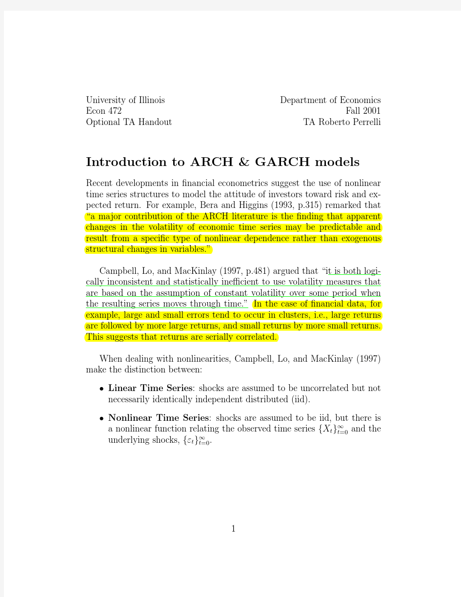
University of Illinois Department of Economics Econ472Fall2001 Optional TA Handout TA Roberto Perrelli Introduction to ARCH&GARCH models Recent developments in?nancial econometrics suggest the use of nonlinear time series structures to model the attitude of investors toward risk and ex-pected return.For example,Bera and Higgins(1993,p.315)remarked that “a major contribution of the ARCH literature is the?nding that apparent changes in the volatility of economic time series may be predictable and result from a speci?c type of nonlinear dependence rather than exogenous structural changes in variables.”
Campbell,Lo,and MacKinlay(1997,p.481)argued that is both logi-cally inconsistent and statistically ine?cient to use volatility measures that are based on the assumption of constant volatility over some period when the resulting series moves through time.”In the case of?nancial data,for example,large and small errors tend to occur in clusters,i.e.,large returns are followed by more large returns,and small returns by more small returns. This suggests that returns are serially correlated.
When dealing with nonlinearities,Campbell,Lo,and MacKinlay(1997) make the distinction between:
?Linear Time Series:shocks are assumed to be uncorrelated but not necessarily identically independent distributed(iid).
?Nonlinear Time Series:shocks are assumed to be iid,but there is
a nonlinear function relating the observed time series{X t}∞
t=0and the
underlying shocks,{εt}∞
t=0
.
1
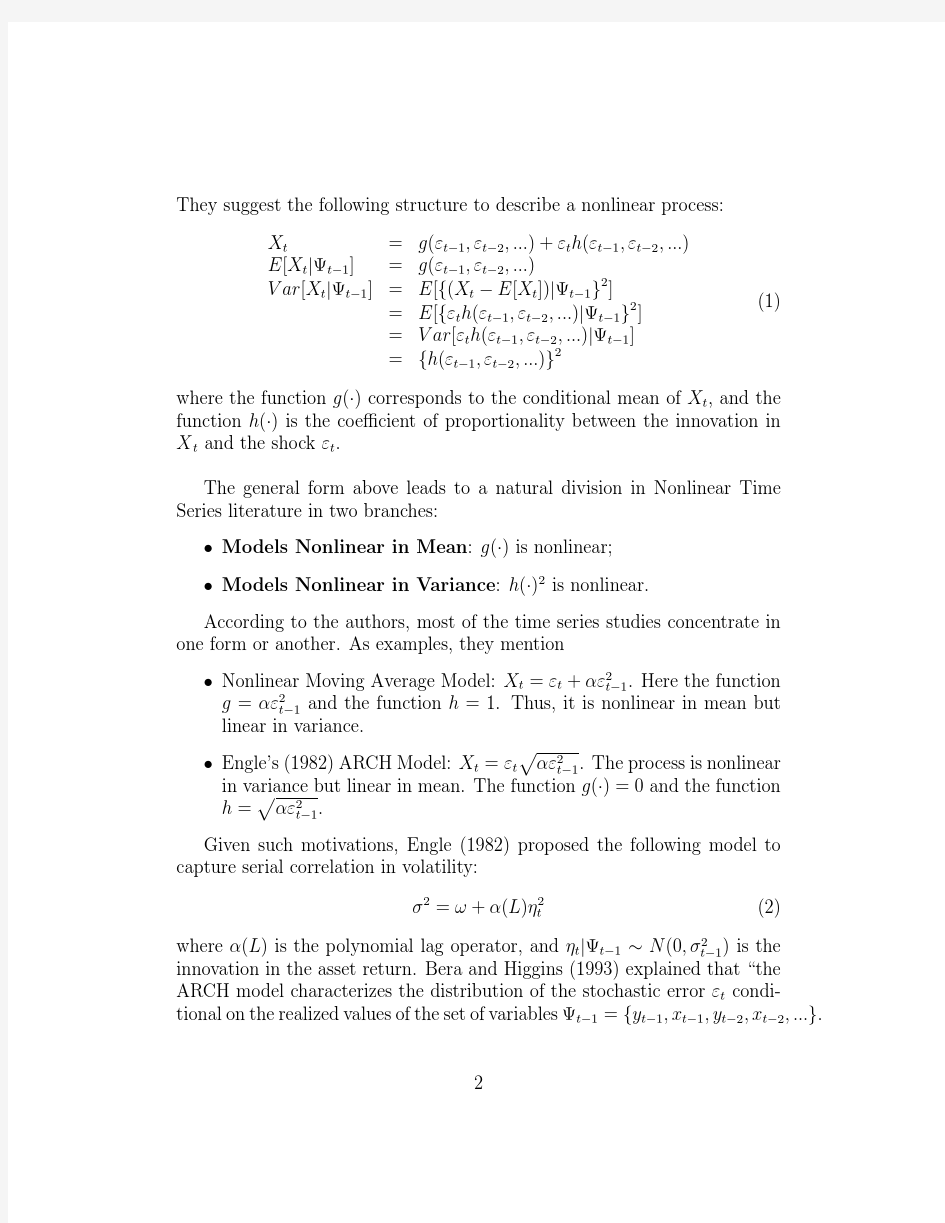
They suggest the following structure to describe a nonlinear process:
X t =g (εt ?1,εt ?2,...)+εt h (εt ?1,εt ?2,...)
E [X t |Ψt ?1]=g (εt ?1,εt ?2,...)
V ar [X t |Ψt ?1]=E [{(X t ?E [X t ])|Ψt ?1}2]
=E [{εt h (εt ?1,εt ?2,...)|Ψt ?1}2]
=V ar [εt h (εt ?1,εt ?2,...)|Ψt ?1]
={h (εt ?1,εt ?2,...)}2(1)
where the function g (·)corresponds to the conditional mean of X t ,and the function h (·)is the coe?cient of proportionality between the innovation in X t and the shock εt .
The general form above leads to a natural division in Nonlinear Time Series literature in two branches:
?Models Nonlinear in Mean :g (·)is nonlinear;
?Models Nonlinear in Variance :h (·)2is nonlinear.
According to the authors,most of the time series studies concentrate in one form or another.As examples,they mention
?Nonlinear Moving Average Model:X t =εt +αε2t ?1.Here the function g =αε2t ?1and the function h =1.Thus,it is nonlinear in mean but linear in variance.
?Engle’s (1982)ARCH Model:X t =εt αε2t ?1.The process is nonlinear
in variance but linear in mean.The function g (·)=0and the function h = αε2t ?1.
Given such motivations,Engle (1982)proposed the following model to capture serial correlation in volatility:
σ2=ω+α(L )η2t (2)
where α(L )is the polynomial lag operator,and ηt |Ψt ?1~N (0,σ2t ?1)is the
innovation in the asset return.Bera and Higgins (1993)explained that “the ARCH model characterizes the distribution of the stochastic error εt condi-tional on the realized values of the set of variables Ψt ?1={y t ?1,x t ?1,y t ?2,x t ?2,...}.
2
Computational problems may arise when the polynomial presents a high order.To facilitate such computation,Bollerslev(1986)proposed a Gener-alized Autorregressive Conditional Heteroskedasticity(GARCH)model,
σ2 t =ω+β(L)σ2
t?1
+α(L)η2
t
(3)
It is quite obvious the similar structure of Autorregressive Moving Average (ARMA)and GARCH processes:a GARCH(p,q)has a polynomialβ(L)
of order“p”-the autorregressive term,and a polynomialα(L)of order“q”
-the moving average term.
Properties and Interpretations of ARCH Models
Following Bera and Higgins(1993),two important concepts should be intro-duced at this point:
De?nition1(Law of Iterated Expectations):Let?1and?2be two sets
of random variables such that?1??2.Let Y be a scalar random variable. Then,E[Y|?1]=E[E[Y|?2]|?1].
Note(Conditionality versus Inconditionality):If?1=?,then E[E[Y|?2]]= E[Y].
Without loss of generality,let a ARCH(1)process be represented by
u t=εt
α0+α1u2
t?1
(4)
where{εt}∞
t=0is a white noise stochastic process.Johnston and DiNardo
(1997)brie?y mention the following properties of ARCH models:?u t have mean zero.
Proof:
u t=εt
α0+α1u2
t?1
E t?1[u t]=E t?1[εt]
α0+α1u2
t?1
=0
E t?2E t?1[u t]=0
(...)
E[u t]=0
(5)
3
?u t have conditional variance given byσ2
t =α0+α1u2
t?1
.
Proof:
u2 t =ε2
t
[α0+α1u2
t?1
]
E t?1[u2
t ]=σ2
ε
[α0+α1u2
t?1
]
=1[α0+α1u2
t?1
]
=σ2
t
(6)
?u t have unconditional variance given byσ2=α0
1?α1.
Proof:
E t?2E t?1[u2
t ]=E t?2[α0+α1u2
t?1
]
=α0+α1E t?2[u2
t?1
]
=α0+α0α1+α2
1
u2
t?2
E t?3E t?2E t?1[u2
t ]=E t?3[α0+α0α1+α2
1
u2
t?2
]
=α0+α0α1+α2
1
E t?3[u2
t?2
]
=α0+α0α1+α0α2
1
+α3
1
u t?3
(...)
E0E1E2(...)E t?2E t?1[u2
t ]=α0(1+α1+α2
1
+...+αt?1
1
)+αt
1
u2
0 =α0
1?α1
=σ2
(7)
Therefore,unconditionally the process is Homoskedastic.
?u t have zero-autocovariances.
Proof:
E t?1[u t u t?1]=u t?1E t?1[u t]=0(8)
Regarding kurtosis,Bera and Higgins(1993)show that the process has a heavier tail than the Normal distribution,given that
E[ε4
t
]
σ4
ε=3(
1?α2
1
1?3α2
1
)>3(9)
Heavy tails are a common aspect of?nancial data,and hence the ARCH models are so popular in this?eld.Besides that,Bera and Higgins(1993) mention the following reasons for the ARCH success:
4
?ARCH models are simple and easy to handle
?ARCH models take care of clustered errors
?ARCH models take care of nonlinearities
?ARCH models take care of changes in the econometrician’s ability to forecast
In fact,the last aspect was pointed by Engle(1982)as a“random coe?-cients”problem:the power of forecast changes from one period to another.
In the history of ARCH literature,interesting interpretations of process can be found.E.g.:
?Lamoureux and Lastrapes(1990).They mention that the conditional heteroskedasticity may be caused by a time dependence in the rate of information arrival to the market.They use the daily trading volume of stock markets as a proxy for such information arrival,and con?rm its signi?cance.
?Mizrach(1990).He associates ARCH models with the errors of the economic agents’learning processes.In this case,contemporaneous errors in expectations are linked with past errors in the same expec-tations,which is somewhat related with the old-fashioned“adaptable expectations hypothesis”in macroeconomics.
?Stock(1998).His interpretation may be summarized by the argument that“any economic variable,in general,evolves an on‘operational’time scale,while in practice it is measured on a‘calendar’time scale.And this inappropriate use of a calendar time scale may lead to volatility clustering since relative to the calendar time,the variable may evolve more quickly or slowly”(Bera and Higgins,1990,p.329;Diebold, 1986].
Estimating and Testing ARCH Models
Johnston and DiNardo(1997)suggest a very simple test for the presence of ARCH problems.The basic menu(step-by-step)is:
?Regress y on x by OLS and obtain the residuals{εt}.
5
?Compute the OLS regressionε2
t =?α0+?α1ε2
t?1
+...+?αpε2
t?p
+error.
?Test the joint signi?cance of?α1,...,?αp.
In case that any of the coe?cients are signi?cant,a straight-forward method of estimation(correction)is provided by Greene(1997).It consists in a four-step FGLS:
?Regress y on x using least squares to obtain?βandεvectors.
?Regressε2
t on a constant andε2
t?1
to obtain the estimates ofα0andα1,
using the whole sample(T).Denote[?α0,?α1]=?→α.
?Compute f t=?α0+?α1ε2
t?1.Then compute the asymptotically e?-
cient estimate?α,?α=?→α+dα,where dαis the least squares coe?cient vector in the regression
[(ε2
t
f t
)?1]=?z0(
1
f t
)+?z1(
ε2
t?1
f t
)+error(10)
The asymptotic covariance matrix for?αis2(?z ?z)?1,where?z is the regressor vector in this regression.
?Recompute f t using?α;then compute
r t=[1
f t +2(?α1εt
f t+1
)2]1/2
s t=1
f t ??α1
f t+1
[ε2t+1
f t+1
?1]
(11)
Compute the estimate?β=?→
β+dβ,where dβis the least squares
coe?cient vector in the regression
[εt s t
r t
]=?wx t r t+error(12)
The asymptotic covariance matrix for?βis given by(?w ?w)?1,where?w is the regressor vector on the equation above.
6
References
[1]Bera,A.K.,and Higgins,M.L.(1993),“ARCH Models:Properties,
Estimation and Testing,”Journal of Economic Surveys,Vol.7,No.4, 307-366.
[2]Bollerslev,T.(1986),“Generalized Autorregressive Conditional Het-
eroskedasticity,”Journal of Econometrics,31,307-327.
[3]Campbell,J.Y.,Lo,A.W.,and MacKinlay,A.C.(1997),The Econo-
metrics of Financial Markets,Princeton,New Jersey:Princeton Uni-versity Press.
[4]Diebold,F.X.(1986),“Modelling the persistence of Conditional Vari-
ances:A Comment,”Econometric Reviews,5,51-56.
[5]Engle,R.(1982),“Autorregressive Conditional Heteroskedasticity with
Estimates of United Kingdom In?ation”,Econometrica,50,987-1008.
[6]Greene,W.(1997),Econometric Analysis,Third Edition,New Jersey:
Prentice-Hall.
[7]Johnston,J.,and DiNardo,J.(1997),Econometric Methods,Fourth
Edition,New York:McGraw-Hill.
[8]Lamoureux,G.C.,and Lastrapes,W.D.(1990),“Heteroskedasticity
in Stock Return Data:Volume versus GARCH E?ects,”Journal of Fi-nance,45,221-229.
[9]Mizrach,B.(1990),“Learning and Conditional Heteroskedasticity in
Asset Returns,”Mimeo,Department of Finance,The Warthon School, University of Pennsylvania.
[10]Stock,J.H.(1988),“Estimating Continuous-Time Processes Subject
to Time Deformation,”Journal of the American Statistical Association (JASA),83,77-85.
7
