3D Face Recognition

Abstract —Recently, a 3D face recognition approach based on geometric invariant signatures, has been proposed. The key idea of the algorithm is a representation of the facial surface, invariant to isometric deformations, such as those resulting from facial expressions. One of the crucial stages in the construction of the geometric invariants is the measurement of geodesic distances on triangulated surfaces, carried out by fast marching on triangulated domains (FMTD). Proposed here is a method, which uses only the metric tensor of the surface for geodesic distance computation. When combined with photometric stereo used for facial surface acquisition, it allows constructing a bending-invariant representation of the face without reconstructing the 3D surface.

Index Terms --face recognition, fast marching, photometric stereo, multidimensional scaling.

I. I NTRODUCTION

ACE recognition is a biometric method that unlike other biometrics, is non-intrusive and can be used even without the subject’s knowledge. State-of-the-art face recognition systems are based on a 40-year heritage of 2D algorithms, dating back to the early 1960s [1]. The first face recognition methods used the geometry of key points (like the eyes, nose and mouth) and their geometric relationships (angles, lengths, ratios, etc.). In 1991, Turk and Pentland applied principal component analysis (PCA) to face imaging [2]. This has become known as the eigenface algorithm and is now a golden standard in face recognition. Later, algorithms inspired by eigenfaces that use similar ideas were proposed (see [3], [4], [5]).

However, all the 2D (image-based) face recognition methods appear sensitive to illumination conditions, head orientations, facial expressions and makeup. These limitations of 2D methods stem directly from the limited information about the face contained in a 2D image. Recently, it became evident that the use of 3D data of the face can be of great help as 3D information is viewpoint and lighting-condition independent, i.e. lacks the “intrinsic” weaknesses of 2D

approaches.

Gordon showed that combining frontal and profile views can improve recognition accuracy [6]. This idea was extended Alexander (alexbron@https://www.sodocs.net/doc/e43159955.html,) and Michael Bronstein (bronstein@https://www.sodocs.net/doc/e43159955.html,) are with the Department of Electrical Engineering, Technion. Ron Kimmel

(ron@cs.technion.ac.il) and Alon Spira (salon@cs.technion.ac.il) are with the

Department of Computer Science, Technion.

by Beumier and Acheroy, who compared central and lateral profiles from the 3D facial surface, acquired by a structured light range camera [7]. This approach demonstrated better robustness to head orientations. Another attempt to cope with the problem of head pose was presented by Huang et al . using 3D morphable head models [8]. Mavridis et al . incorporated a range map of the face into the classical face recognition algorithms based on PCA and hidden Markov models [9]. Particularly, this approach showed robustness to large variations in color, illumination and use of cosmetics, and also allowed separating the face from a cluttered background.

However, none of the approaches proposed heretofore was able to overcome the problems resulting from the non-rigid nature of the human face. For example, Beumier and Acheroy failed to perform accurate global surface matching, and observed that the recognition accuracy decreased when too many profiles were used [7]. The difficulty in performing accurate surface matching of facial surfaces was one of the primary limiting factors of other 3D face recognition algorithms as well.

An attempt to overcome these difficulties has been recently proposed in [10], using the bending invariant canonical forms [11]. In this approach, the facial surface is converted into a representation, which is practically identical for different postures of the face. One of the key stages in the construction of the bending invariant representation is the computation of the geodesic distances between points on a triangulated manifold.

In this work, we present a variation of fast marching on triangulated domains (FMTD), capable of computing geodesic distances given only the metric tensor of the surface. We propose to combine this algorithm with the photometric stereo method for facial surface acquisition. Photometric stereo is a cheap and simple approach, producing the metric tensor without reconstructing the surface. As the result, a simple and fast face recognition method is obtained.

II. S URFACE A CQUISITION

The face recognition algorithm discussed in this paper treats faces as three-dimensional surfaces. It is therefore necessary to

obtain first the facial surface of the subject that we are trying

to recognize. Here, we focus on methods, that produce the surface gradient. As it will be shown in Section IV, the actual surface reconstruction is not needed, saving computational effort and reducing numerical errors. 3D Face Recognition without Facial Surface

Reconstruction

Alexander M. BRONSTEIN, Michael M. BRONSTEIN, Ron KIMMEL and Alon SPIRA

F

T e c h n i o n - C o m p u t e r S c i e n c e D e p a r t m e n t - T e c h n i c a l R e p o r t C I S -2003-05 - 2003

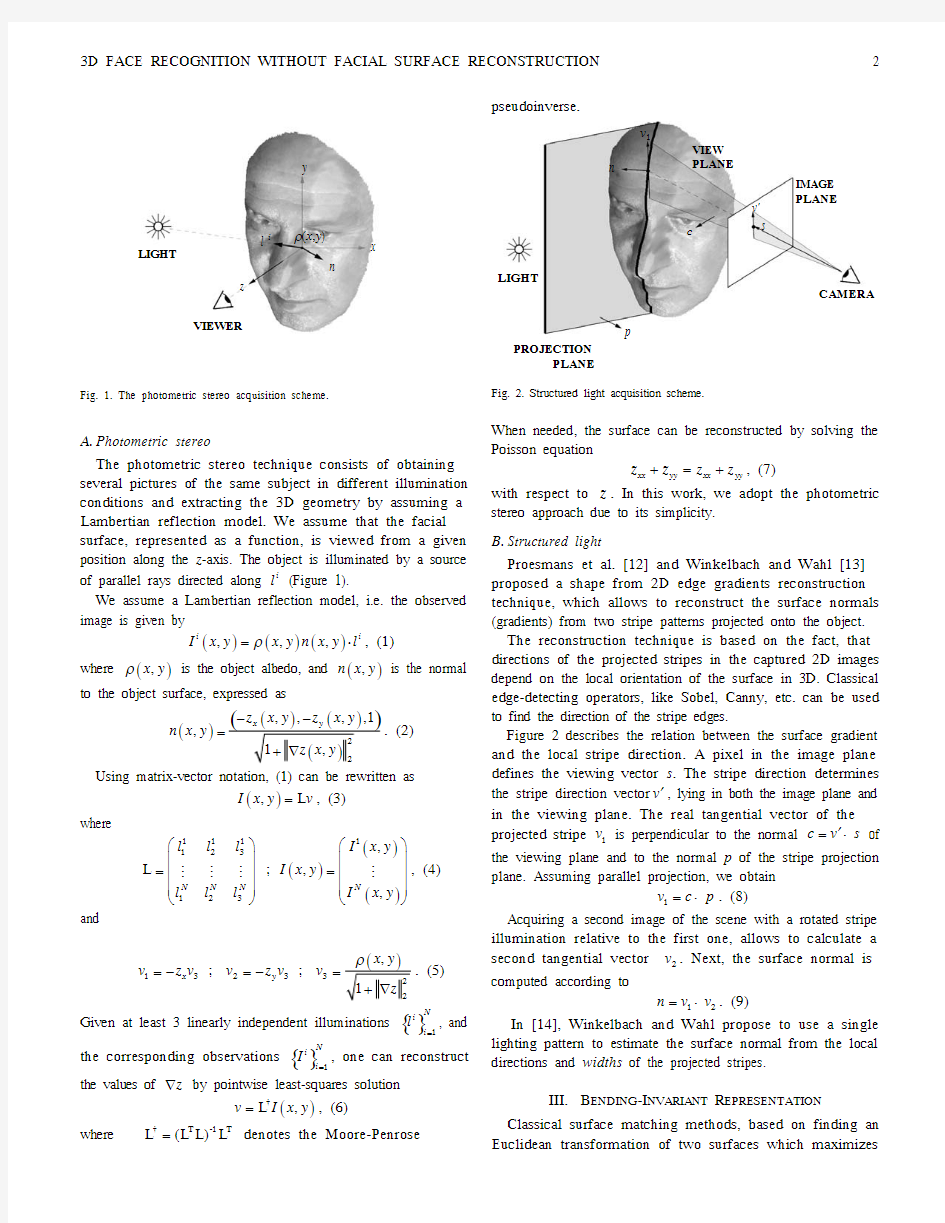
Fig. 1. The photometric stereo acquisition scheme.

A. Photometric stereo

The photometric stereo technique consists of obtaining several pictures of the same subject in different illumination

conditions and extracting the 3D geometry by assuming a

Lambertian reflection model. We assume that the facial

surface, represented as a function, is viewed from a given position along the z -axis. The object is illuminated by a source of parallel rays directed along i

l (Figure 1). We assume a Lambertian reflection model, i.e. the observed image is given by ()()(),,,i i

I x y x y n x y l ρ=?, (1)

where (),ρx y is the object albedo, and (),n x y is the normal

to the object surface, expressed as ()

,,,,1,z x y z x y n x y ??=. (2) Using matrix-vector notation, (1) can be rewritten as

(),L I x y v =, (3) where

()()()111

1123

123,L ;

,,N N N N l l l I x y I x y l l l I x y ????????

==????????????

##

##, (4) and

13233, ; ; x y x y v z v v z v v =?=?=. (5) Given at least 3 linearly independent illuminations {}1

N

i i l =, and the corresponding observations {}1

=N

i i I , one can reconstruct the values of ?z by pointwise least-squares solution

()?L ,v I x y =, (6)

where ?T -1T L (L L)L = denotes the Moore-Penrose

pseudoinverse.

Fig. 2. Structured light acquisition scheme.

When needed, the surface can be reconstructed by solving the

Poisson equation

xx yy xx yy z z z z +=+ , (7) with respect to z

. In this work, we adopt the photometric stereo approach due to its simplicity.

B. Structured light Proesmans et al. [12] and Winkelbach and Wahl [13]

proposed a shape from 2D edge gradients reconstruction technique, which allows to reconstruct the surface normals (gradients) from two stripe patterns projected onto the object.

The reconstruction technique is based on the fact, that directions of the projected stripes in the captured 2D images

depend on the local orientation of the surface in 3D. Classical

edge-detecting operators, like Sobel, Canny, etc. can be used

to find the direction of the stripe edges. Figure 2 describes the relation between the surface gradient and the local stripe direction. A pixel in the image plane defines the viewing vector s . The stripe direction determines the stripe direction vector v ′, lying in both the image plane and in the viewing plane. The real tangential vector of the

projected stripe 1v is perpendicular to the normal c v s ′=× of the viewing plane and to the normal p of the stripe projection plane. Assuming parallel projection, we obtain

1v c p =×. (8) Acquiring a second image of the scene with a rotated stripe illumination relative to the first one, allows to calculate a

second tangential vector 2v . Next, the surface normal is computed according to 12n v v =×. (9)

In [14], Winkelbach and Wahl propose to use a single lighting pattern to estimate the surface normal from the local directions and widths of the projected stripes.

III. B ENDING -I NVARIANT R EPRESENTATION Classical surface matching methods, based on finding an

Euclidean transformation of two surfaces which maximizes x

z

y

l i

n

LIGHT ρ(x ,y )

VIEWER

PROJECTION

PLANE

c

v'

s

p

v 1

n

VIEW PLANE

IMAGE PLANE

CAMERA

LIGHT

T e c h n i o n - C o m p u t e r S c i e n c e D e p a r t m e n t - T e c h n i c a l R e p o r t C I S -2003-05 - 2003

some shape similarity criterion (see, for example, [15], [16], [17]), are suitable mainly for rigid objects. Human face can by

no means be considered as a rigid object since it undergoes

deformations resulting from facial expressions. On the other hand, the class of transformations that a facial surface can undergo is not arbitrary, and empirical observations show that facial expressions can be modeled as isometric (or length-preserving) transformations. Such transformations do not stretch and not do they tear the surface, or more rigorously, preserve the surface metric. The surfaces resulting from such transformations are called isometric surfaces . The requirement from a deformable surface matching algorithm is to find a representation, which is the same for all isometric surfaces. Schwartz et al. were the first to introduce the use of multidimensional scaling (MDS) as a tool for studying curved surfaces by planar models [18]. Zigelman et al. [19] and Grossman et al. [20] extended some of these ideas to the problem of texture mapping and voxel-based cortex flattening. A generalization of this approach was introduced in the recent work of Elad and Kimmel [11], as a framework for object recognition. They showed an efficient algorithm for constructing a representation of surfaces, invariant under isometric transformations. This method, referred to as bending-invariant canonical forms, is the core of our 3D face recognition framework.

Let us be given a polyhedral approximation of the facial surface, S. One can think of such an approximation as if obtained by sampling the underlying continuous surface on a finite set of points p i (i = 1,…,n ), and discretizing the metric δ associated with the surface

()i j ij δp ,p =δ. (10) Writing the values of δij in matrix form, we obtain the matrix of mutual distances between the surface points. For convenience, we define the squared mutual distances,

()2ij ij =δΔ. (11)

The matrix Δ is invariant under isometric surface deformations, but is not a unique representation of isometric surfaces, since it depends on arbitrary ordering and the selection of the surface points. We would like to obtain a geometric invariant, which would be unique for isometric

surfaces on one hand, and will allow using simple rigid surface matching algorithms to compare such invariants on the other. Treating the squared mutual distances as a particular case of dissimilarities , one can apply a dimensionality-reduction technique called multidimensional scaling (MDS) in order to embed the surface into a low-dimensional Euclidean space R m . This is equivalent to finding a mapping between two metric spaces,

()()():S,R , ; m i i d p x ?δ?→=, (12) that minimizes the embedding error,

()

2 ; ij ij ij i j f d d x x εδ=?=?, (13) for some monotone function f that sums over all ij . The obtained m -dimensional representation is a set of points x i ∈ R m (i = 1,…,n ), corresponding to the surface points p i . Different MDS methods can be derived using different embedding error criteria [21].

A particular case is the classical scaling , introduced by Young and Householder [22]. The embedding in R m is performed by double-centering the matrix Δ 12

B J J =?Δ (14) (here J = I - 1n

U; I is a n ×n identity matrix, and U is a matrix consisting entirely of ones). The first m eigenvectors e i , corresponding to the m largest eigenvalues of B, are used as the embedding coordinates ; =1,...,; =1,...,j j i i x e i n j m =, (15) where j i x denotes the j -th coordinate of the vector x i . We refer to the set of points x i obtained by the MDS as the bending-invariant canonical form of the surface; when m =3, it can be plotted as a surface. Standard rigid surface matching methods can be used in order to compare between two deformable surfaces, using their bending-invariant representations instead of the surfaces themselves. Since the canonical form is computed up to a translation, rotation, and reflection transformation, to allow comparison between canonical forms, they must be aligned . This can be done, for instance, by setting the first-order moments (center of mass) and the mixed second-order moments to zero (see [23]).

IV. M EASURING G EODESIC D ISTANCES

One of the crucial steps in the construction of the canonical form of a given surface, is an efficient algorithm for the computation of geodesic distances on surfaces, that is, δij . A

numerically consistent algorithm for distance computation on

triangulated domains, henceforth referred to as fast marching on triangulated domains (FMTD), was used by Elad and

Kimmel [11]. FMTD was proposed by Kimmel and Sethian [24] as a generalization of the fast marching method [25].

Using FMTD, the geodesic distances between a surface vertex

and the rest of the n surface vertices can be computed in O(n ) operations. Measuring distances on manifolds was also done before for graphs of functions [26] and implicit manifolds [27].

Since the main focus of this paper is how to avoid the surface reconstruction, we present a modified version of FMTD, which computes the geodesic distances on a surface, using the values of the surface gradient ?z only. These values can be obtained, for example, from photometric stereo or structured light.

The facial surface can be thought of as a parametric manifold, represented by a mapping 23X :→R R from the parameterization plane ()()12U ,,u u x y == to the parametric manifold

()()()()()

112212312X U ,,,,,x u u x u u x u u =; (16)

which, in turn, can be written as

()()()X U ,,,x y z x y =. (17) T e c h n i o n - C o m p u t e r S c i e n c e D e p a r t m e n t - T e c h n i c a l R e p o r t C I S -2003-05 - 2003

Fig. 3. The orthogonal grid on the parameterization plane U is transformed

into a non-orthogonal one on the manifold X(U).

The derivatives of X with respect to u i are defined as

X i

i u X ??=, and they constitute a non-orthogonal coordinate system on the manifold (Figure 3). In the particular case of (17),

()()121,0,, 0,1,x y X z X z ==. (18) The distance element on the manifold is

ds =, (19) where we use Einstein’s summation convention, and the metric tensor g ij of the manifold is given by ()11121112212221

22ij g g X X X X g g g X X X X ??????

==??????????. (20) The classical fast marching method [25] calculates distances in an orthogonal coordinate system. The numerical stencil for the update of a grid point consists of the vertices of a right triangle. In our case, 120g ≠ and the resulting triangles are not necessarily right ones. If a grid point is updated by a stencil

which is an obtuse triangle, a problem may arise. The values of one of the points of the stencil might not be set in time and cannot be used. There is a similar problem with fast marching on triangulated domains which include obtuse triangles [24]. Our solution is similar to that of [24]. We perform a preprocessing stage for the grid, in which we split every obtuse triangle into two acute ones (see Figure 4). The split is performed by adding an additional edge, connecting the updated grid point with a non-neighboring grid point. The distant grid point becomes part of the numerical stencil. The need for splitting is determined according to the angle between the non-orthogonal axes at the grid point. It is calculated by

121

2cos X X X X α???==??????If cos 0α=, the axes are perpendicular, and no splitting is

required. If cos 0α<, the angle α is obtuse and should be split. The denominator of (21) is always positive, so we need only check the sign of the numerator 12g . In order to split an angle, we should connect the updated grid point with another

point, located m grid points from the point in the X 1 direction,

and n grid points in the X 2 direction (m and n can be negative).

Fig. 4 The numerical support for the non-orthogonal coordinate system.

Triangle 1 gives a proper numerical support, yet triangle 2 is obtuse. It is

replaced by triangle 3 and triangle 4.

The point is a proper supporting point, if the obtuse angle is

split into two acute ones. For cos 0α< this is the case if ()

11211

12cos 0

X mX nX X mX nX β??

?+==????+??=> (22)

and

()

21222

12cos 0.X mX nX X mX nX β??

?+==

????

+??=> (23)

Also, here it is enough to check the sign of the numerators. For cos 0α>, 2cos β changes its sign and the constraints are 111212220, 0mg ng mg ng +>+<. (24) This process is done for all grid points. Once the preprocessing stage is done, we have a suitable numerical stencil for each grid point and we can calculate the distances. The numerical scheme used is similar to that of [24], with the exception that there is no need to perform the unfolding step. The supporting grid points that split the obtuse angles can be found more efficiently. The required triangle edge lengths and angles are calculated according to the surface metric g ij at the grid point, which, in turn, is computed using the surface

gradients x z , y z . A more detailed description appears in [28]. V. 3D F ACE R ECOGNITION As a first step, the 3D face recognition system acquires the surface gradient ?z, as discussed in Section II. At the second stage, the raw data are preprocessed. Preliminary processing,

such as centering and cropping can be carried out by simple

pattern matching, which can use the eyes as the most

recognizable feature of the human face.

1X

u 1

u 2

X 2

X 1

T e c h n i o n - C o m p u t e r S c i e n c e D e p a r t m e n t - T e c h n i c a l R e p o r t C I S -2003-05 - 2003

(0°,0°) (0°,-20°) (0°,+20°) (-25°,0°) (+25°,0°)

Fig. 5. Different illuminations of the face. Numbers in brackets indicate the azimuth and the elevation angle, respectively, determining the illumination direction.

The facial contour should also be extracted in order to limit the processing to the surface belonging only to the face itself. Preprocessing should emphasize those sections of the face less susceptible to alteration and exclude the parts that can be easily changed (e.g. hair). In this work, the preprocessing stage was limited to cropping the triangulated manifold by removing the parts lying outside an ellipse (in the geodesic sense) centered at the nose tip.

Next, an n ×n matrix of geodesic distances is created by applying FMTD from each of the n selected vertices. Then, MDS is applied to the distance matrix, producing a canonical form of the face in a low-dimensional Euclidean space (three-dimensional in all our experiments).

The canonical form obtained this way is compared with a database of templates corresponding to other subjects (one-to-many match), or to a single stored template (one-to-one match). If the correspondence of the compared canonical form falls within a certain statistical range of values, the match is considered to be valid.

Finding correspondence between the canonical forms is a problem by itself and brings us back to the surface matching problem. However, the major difference here is the fact that the matching is performed between the rigid canonical forms carrying the intrinsic object geometry, rather than the deformable facial surfaces themselves. Thus even the simplest rigid surface matching algorithms produce plausible results. In this work, we adopted the moments [23] due to its simplicity. The canonical form’s (p, q, r )-th moment is given by

()()()1

23p q r pqr n n n n

M x x x =∑ (25)

where i

n x denotes the i th coordinate of the n th point in the canonical surface samples. In order to compare between two

canonical forms, the vector ()111

,...,M

M M

p q r p q r M M , termed as the

moments signature , is computed for each surface. The

Euclidean distance between two moments signatures measures the dissimilarity between the two surfaces.

VI. E XPERIMENTAL R ESULTS

We performed an experiment, which demonstrates that

comparison of canonical forms obtained without actual facial surface reconstruction is better than reconstruction and direct comparison of the surfaces. The Yale Face Database B [29]

was used. The database consisted of high-resolution grayscale

images of different instances of 10 subjects of both Caucasian

bending-invariant canonical form represented as a surface (right).

and Asian type, taken in controlled illumination conditions (Figure 5). Some instances of 7 subjects were taken from the database for the experiment.

Direct surface matching consisted of the retrieval of the surface gradient according to (6) using 5 different illumination directions, reconstruction of the surface according to (7), alignment and computation of the surface moments signature according to (25). Canonical forms were computed from the surface gradient, aligned and converted into a moment signature according to (25).

In order to get some impression of the algorithms accuracy, we converted the relative distances between the subjects produced by each algorithm into 3D proximity patterns (Figure 7). These patterns, representing each subject as a point in R 3, were obtained by applying MDS to the relative distances (with a distortion less than 1%).

The entire cloud of dots was partitioned into clusters formed by instances of the subjects C 1―C 7. Visually, the more C i are compact and distant from other clusters, the more accurate is the algorithm. Quantitatively, we measured (i) the variance σi of C i and (ii) the distance d i between the centroid of C i and the centroid of the nearest cluster.

Table I shows a quantitative comparison of the algorithms. Inter-cluster distances d i are given in units of the variance σi . Clusters C 5―C 7, consisting of a single instance of the subject are not presented in the table. The use of canonical forms

improved the cluster variance and the inter-cluster distance by about one order of magnitude, compared to direct facial

surface matching.

TABLE I F ACE R ECOGNITION A CCURACY

CLUSTER

σDIRECT d DIRECT

σCANONICAL

d CANONICAL

C 1 0.1749 0.1704 0.0140 4.3714 C 2 0.2828 0.3745 0.0120 5.1000 C 3

0.0695 0.8676 0.0269 2.3569

C 4 0.0764 0.7814 0.0139 4.5611 VII. C ONCLUSIONS We have shown how to perform 3

D face recognition

according to [10], without reconstructing the facial surface.

T e c h n i o n - C o m p u t e r S c i e n c e D e p a r t m e n t - T e c h n i c a l R e p o r t C I S -2003-05 -

Fig. 7. Visualization of the face recognition results as three-dimensional proximity patterns. Subjects from the face database represented as points obtained by applying MDS to the relative distances between subjects. Shown here: straightforward surface matching (A) and canonical forms (B).

3D face recognition based on bending-invariant representations, unlike previously proposed solutions, makes face recognition robust to facial expressions, head orientations and illumination conditions. Our approach shown here allows

an efficient use of simple 3D acquisition techniques (e.g.

photometric stereo) for fast and accurate face recognition. Experimental results demonstrate superiority of our approach

over straightforward rigid surface matching.

R EFERENCES [1] W. W. Bledsoe, The model method in facial recognition. Technical

report PRI 15, Panoramic Research Inc., Palo Alto , 1966.

[2] M. Turk and A.. Pentland,, Face recognition using eigenfaces, Proc.

CVPR , pp. 586-591, 1991.

[3] V. I. Belhumeur, J. P. Hespanha and D. J. Kriegman, Eigenfaces vs.

Fisherfaces: recognition using class specific linear projection, IEEE

Trans. PAMI 19(7), pp. 711-720, 1997.

[4] B. J. Frey, A. Colmenarez and T. S. Huang, Mixtures of local linear

subspaces for face recognition, Proc. CVPR , pp. 32-37, 1998.

[5] B. Moghaddam, T. Jebara and A. Pentland, Bayesian face recognition.

Technical Report TR2000-42, Mitsubishi Electric Research Laboratories, 2000.

[6] G. Gordon, Face recognition from frontal and profile views, Proc. Int’l Workshop on Face and Gesture Recognition , pp. 47-52, 1996.

[7] C. Beumier and M. P. Acheroy, Automatic face authentication from 3D surface , Proc. British Machine Vision Conf. (BMVC), pp 449-458,

1998.

[8] J. Huang, V. Blanz and B. Heisele, Face recognition using component-based SVM classification and morphable models, SVM 2002, pp. 334-341, 2002.

[9] N. Mavridis, F. Tsalakanidou, D. Pantazis, S. Malassiotis and M. G.

Strintzis, The HISCORE face recognition application: Affordable

desktop face recognition based on a novel 3D camera, Proc. Int’l Conf.

on Augmented Virtual Environments and 3D Imaging (ICAV3D),

Mykonos, Greece, 2001.

[10] Anonymous authors, 3D face recognition using geometric invariants,

Submitted for publication 2003.

[11] A. Elad, R. Kimmel, Bending invariant representations for surfaces,

Proc. CVPR , pp. 168-174, 2001.

[12] M. Proesmans, L. Van Gool and A. Oosterlinck, One-shot active shape

acquisition, Proc. Internat. Conf. Pattern Recognition , Vienna, Vol. C,

pp. 336- 340, 1996.

[13] S. Winkelbach and F. M. Wahl, Shape from 2D edge gradients, Pattern

Recognition, Lecture Notes in Computer Sciences 2191, pp. 377-384,

Springer, 2001.

[14] S. Winkelbach and F. M. Wahl, Shape from single stripe pattern

illumination, L. Van Gool (Ed): Pattern Recognition (DAGM 2002), Lecture Notes in Computer Science 2449, pp. 240-247, Springer, 2002. [15] O. D. Faugeras and M. Hebert, A 3D recognition and positioning

algorithm using geometrical matching between primitive surfaces, Proc.

7th Int’l Joint Conf. on Artificial Intelligence , pp. 996–1002, 1983. [16] P. J. Besl, The free form matching problem. Machine vision for three-dimensional scene , In: Freeman, H. (ed.) New York Academic , 1990. [17] G. Barequet and M. Sharir, Recovering the position and orientation of

free-form objects from image contours using 3D distance map , IEEE

Trans. PAMI , 19(9), pp. 929–948, 1997. [18] E. L. Schwartz, A. Shaw and E. Wolfson, A numerical solution to the generalized mapmaker's problem: flattening nonconvex polyhedral surfaces, IEEE Trans. PAMI , 11, pp. 1005-1008, 1989. [19] G. Zigelman, R. Kimmel and N. Kiryati, Texture mapping using surface flattening via multi-dimensional scaling, IEEE Trans. Visualization and Comp. Graphics , 8, pp. 198-207, 2002. [20] R. Grossman, N. Kiryati and R. Kimmel, Computational surface flattening: a voxel-based approach, IEEE Trans. PAMI , 24, pp. 433-441, 2002. [21] I. Borg and P. Groenen, Modern multidimensional scaling - theory and

applications , Springer, 1997. [22] G. Young and G. S. Householder, Discussion of a set of points in terms

of their mutual distances, Psychometrika 3, pp. 19-22, 1938. [23] A. Tal, M. Elad and S. Ar, Content based retrieval of VRML objects –

an iterative and interactive approach”, EG Multimedia , 97, pp. 97-108, 2001. [24] R. Kimmel and J. A. Sethian, Computing geodesic on manifolds. Proc. US National Academy of Science 95, pp. 8431–8435, 1998. [25] J. A. Sethian, A review of the theory, algorithms, and applications of level set method for propagating surfaces. Acta numerica , pp. 309-395, 1996. [26] J. Sethian and A. Vladimirsky, Ordered upwind methods for static Hamilton-Jacobi equations: theory and applications . Technical Report PAM 792 (UCB), Center for Pure and Applied Mathematics, 2001 Submitted for publication to SIAM Journal on Num. Anal., 2001. [27] F. Mémoli and G. Sapiro, Fast computation of weighted distance functions and geodesics on implicit hyper-surfaces. Journal of Computational Physics , 173(2), pp. 730-764, 2001. [28] Anonymous authors, An efficient solution to the eikonal equation on parametric manifolds. Submitted for publication, 2003. [29] Yale Face Database B. Available: https://www.sodocs.net/doc/e43159955.html,/projects/ yalefacesB/yalefacesB.html T e c h n i o n - C o m p u t e r S c i e n c e D e p a r t m e n t - T e c h n i c a l R e p o r t C I S -2003-05 -

ProFace触摸屏GP应用常见问题及处理办法

ProFace触摸屏GP应用常见问题及处理办法 1、CF卡在不同型号GP间是否通用？ 答：通用的。但不是所有品牌的CF卡都能使用。GP目前支持日立、SANDISK、Pro-fac e、金士顿这四种品牌,以上四种经过测试，可行，现在用得比较多的是金士顿，2G的卡也就xxx钱，比Proface的便宜多得多啦。不知道写这样的帖子会不会给我带来麻烦啊-_-! 2、GP内部可否存储数据，掉电以后仍可保留（不通过PLC保存）。 答：可以。在默认状态下GP不具备掉电保持功能，但通过“Back Settings”设置可实现掉电保持。 操作步骤：“GP Setup”-“Extended Settings”-“Back Settings” 设置保存起始地址、存储字数N，在起始地址后的N个字地址均可实现掉电保持。最多可使用6096个字地址（起始地址为LS2096，2000系列），如果使用GP-PRO/PB V 5.05及以前的编辑软件，可使用字地址会减少。 3、趋势图画面可否两个重叠在一起（用于对比显示不同尺度的曲线）？ 答：可以，使用趋势图画面制作两副趋势图画面，在主页面中使用“Lode Screen”功能将２个趋势图画面调入，即可。 （这其中有个问题：当趋势图都选用“笔记录”模式时，显示的画面为一段一段的线段，无法连续，但单一调用一副画面时正常，不解。当选用“正常模式”时,画面显示也正常。） ４、GP进入离线状态可否加密？在哪里设置？ 答：可以，先进入离线状态（OFFLINE），选择“INITIALIZE”，再选择“SYSTEN ENVI RONMENT SETUP”，再选择“SYSTEM SETUP”，然后选择其中的“PASSWORD(0-9999)”一项，在其中输入密码即可。以后每次进入离线状态均需输入密码。需要取消时，将该项设置为０。 在编程软件中，选择“GP Setup”，在“GP Settings”一栏中，在“Password Se tting”后面的框中填入密码，将该程序传入GP内即可。 ５、GP中如何关闭打开背景灯？ 答：背景的打开与关闭可通过系统区来控制。具体控制位：LS001400（直接连接方式）、LS001100（Memory Link方式）。该位为0时背景灯关闭，为1时背景灯打开。 ６、GP和PLC通讯不上是什么原因？ 答：1、确认画面程序中GP型号与PLC型号是否选择正确

工业以太网简介

工业以太网简介: 工业以太网就是基于IEEE 802、3 (Ethernet)得强大得区域与单元网络。利用工业以太网,SIMATIC NET 提供了一个无缝集成到新得多媒体世界得途径。 企业内部互联网(Intranet),外部互联网(Extranet),以及国际互联网(Internet) 提供得广泛应用不但已经进入今天得办公室领域,而且还可以应用于生产与过程自动化。继10M波特率以太网成功运行之后,具有交换功能,全双工与自适应得100M波特率快速以太网(Fast Ethernet,符合IEEE 802、3u 得标准)也已成功运行多年。采用何种性能得以太网取决于用户得需要。通用得兼容性允许用户无缝升级到新技术。 为用户带来得利益 :市场占有率高达80%,以太网毫无疑问就是当今LAN(局域网)领域中首屈一指得网络。以太网优越得性能,为您得应用带来巨大得利益: 通过简单得连接方式快速装配。 通过不断得开发提供了持续得兼容性,因而保证了投资得安全。 通过交换技术提供实际上没有限制得通讯性能。 各种各样联网应用,例如办公室环境与生产应用环境得联网。 通过接入WAN(广域网)可实现公司之间得通讯,例如,ISDN 或Internet 得接入。 SIMATIC NET基于经过现场应用验证得技术,SIMATIC NET已供应多于400,000个节点,遍布世界各地,用于严酷得工业环境,包括有高强度电磁干扰得区域。 工业以太网络得构成 :一个典型得工业以太网络环境,有以下三类网络器件: ◆网络部件 连接部件: ?FC 快速连接插座 ?ELS(工业以太网电气交换机) ?ESM(工业以太网电气交换机) ?SM(工业以太网光纤交换机) ?MC TP11(工业以太网光纤电气转换模块) 通信介质:普通双绞线,工业屏蔽双绞线与光纤 ◆ SIMATIC PLC控制器上得工业以太网通讯外理器。用于将SIMATIC PLC连接到工 业以太网。 ◆ PG/PC 上得工业以太网通讯外理器。用于将PG/PC连接到工业以太网。 工业以太网重要性能:为了应用于严酷得工业环境,确保工业应用得安全可靠,SIMATIC NET 为以太网技术补充了不少重要得性能: ?工业以太网技术上与IEEE802、3/802、3u兼容,使用ISO与TCP/IP 通讯协议?10/100M 自适应传输速率 ?冗余24VDC 供电 ?简单得机柜导轨安装 ?方便得构成星型、线型与环型拓扑结构 ?高速冗余得安全网络,最大网络重构时间为0、3 秒 ?用于严酷环境得网络元件,通过EMC 测试 ?通过带有RJ45 技术、工业级得Sub-D 连接技术与安装专用屏蔽电缆得Fast Connect连接技术,确保现场电缆安装工作得快速进行 ?简单高效得信号装置不断地监视网络元件 ?符合SNMP(简单得网络管理协议) ?可使用基于web 得网络管理 ?使用VB/VC 或组态软件即可监控管理网络。 工业以太网冗余原理

公文命令与决定的区别是什么2篇

公文命令与决定的区别是什么2篇What is the difference between official document order and decision 编订：JinTai College

公文命令与决定的区别是什么2篇 前言：公文是法定机关与组织在公务活动中，按照特定的体式、经过一定的处理程序形成和使用的书面材料，命令是国家行政机关及其领导人发布的指挥性和强制性的公文。本文档根据公文命令内容要求和特点展开说明，具有实践指导意义，便于学习和使用，本文下载后内容可随意调整修改及打印。 本文简要目录如下：【下载该文档后使用Word打开，按住键盘Ctrl键且鼠标单击目录内容即可跳转到对应篇章】 1、篇章1：20xx年公文命令与决定的区别文档 2、篇章2：公文中相似文种的区别文档 公文种类繁多，一不小心就可能弄混，闹出错误。下文是小泰为大家收集的关于命令与决定之间的区别，仅供参考!篇章1:20xx年公文命令与决定的区别文档 一、命令 命令（令）是国家权力机关、行政机关、军事机关及其负责人颁布的，是具有强制执行性质的领导性、指挥性的下行公文。从词义上看，是“使人为事”的意思。“命”还有“严

肃”的含义，“令”有“告诫”的含义。命令是我国最古老的公文文种之一。 三国时候曹操为了完成其统一中国的大业，千方百计广招人才，先后颁布了《求贤令》、《举士令》和《求逸才令》等。在我国古代，命令有称作“誓”、“诰”、“制”、“政”、“策”等的。 命令（令）是“依照有关法律规定发布行政法规和规章;宣布施行重大强制性行政措施;奖惩有关人员;撤销下级机关不适当的决定”时所使用的公文。 二、决定 决定是行政机关对重要事项或重大行动做出具有规定性、强制性和领导、指导性的公文。企事业单位、社会团体使用决定时，其内容应为本机关中相对重要的事宜。一般来说，只有事关全局、政策性强、任务艰巨、执行时间较长的重要工作，才适合使用“决定”行文。 1.指挥性决定。也叫部署性决定，多为对重要事项和重大行动做出部署的决定。这类决定政策性强，要求坚决贯彻执行。

PROFACE触摸屏-配方功能制作方法

PROFACE 触摸屏触摸屏------配方功能配方功能配方功能 配方功能可以允许将多个不同的数据（也就是配方）从触摸屏批量写入PLC 的连续地址中，也可以在触摸屏上编辑后再写入PLC 中去。 现以下面的例子为例，介绍一下配方功能的设置方法。 注： ① 按“读取数据”时，②-配方数据表格内显示项目名，同时“完成指示”灯点亮。 ② 配方数据显示表格-显示配方的项目名称。 ③ “SRAM->PLC ”按钮将配方组合数据从触摸屏写入到PLC ，“PLC->SRAM”按钮PLC 中的配方组合数据写入到触摸屏中。 ④ 上下移动白色方框，选定配方数据表格中显示的项目。 ⑤ 配方组合数据的内容显示。 1、配方设置配方设置

★ 在工程管理器中选择“画面/设置”→“配方数据”→“配方设置”。 ★ 设定配方设置中的内容 注： ① 选择使用配方功能（使用配方功能时，此项必选） ② 写入设置：将配方数据从触摸屏的内存或CF 卡写入SRAM（将配方数据写入到PLC 前必须先写入SRAM） 控制字地址控制字地址：：该字地址的0位为1 时，执行传输动作

写结束位地址写结束位地址：：写入完成后该位为1 ③ PLC 和SRAM 直接传输设置 该功能是由PLC 控制的配方数据自动传输方式，此时必须选中“PLC 控制传输”项。 控制字地址控制字地址：：当PLC 中该字地址的0位为1时，配方数据从SRAM 传到PLC。 传输结束位地址：配方数据传输完成后，此位置1。 2、配方列表设置配方列表设置 ★ 在工程管理器中选择“画面/设置”→“配方数据”→“配方列表”。 ★ 在弹出的“配方数据列表”中，选择配方数据是存于内存还上CF 卡，再点击“添加”。

公文命令与决定有什么不同

公文命令与决定有什么不同 公文种类繁多，一不小心就可能弄混，闹出错误。下文是小雅为大家收集的关于命令与决定的对应范文，仅供参考! 20xx年公文命令与决定的区别 1、制发单位范围。命令的制发单位有明显要求，范围小。只有国家领导机关和领导人、国务院各部门，乡镇以上各级人民政府在他们的本身权限内可以制发命令。其他任何单位和个人不能发布命令，党使用的公文没有命令这种。决定的范围广，上至国家最高行政机关下至地方基层部门都可以使用决定。 2、内容重要性程度不同。命令内容要很重要，不是重大的政策法规、重大的问题与决策、重大的任务与嘉奖一般不用命令。决定一般都是较重要的事项，或有重大行动与活动要安排部署。 3、执行的强制力度不同。命令一经发布，有关下级机关和人员必须无条件地服从与贯彻执行，决不允许延误、怠慢甚至违抗。决定凡决定事项，有关组织、单位和人员要认真贯彻、落实、执行，即使上级做出了很不正确的决定，在上级机关和制发单位未修改之前，有关方面可以提出意见但不能公开对抗，拒绝执行。 命令范文 经股东大会研究决定，自20XX年1月1日起由xxx先生担任杭州xx检测技术有限公司总经理一职，由其全权代理法定代表人负责公司的运行，并定期向股东大会汇报公司的运行情况，以供

股东大会讨论。并授权其任命技术负责人和质量负责人及各部门负责人，具体为： 1. 负责主持本公司行政、技术、业务的全面工作和开展各项质量活动，对本单位的质量管理和工作质量负全责; 2. 负责本公司实验室《质量手册》和程序文件在本单位的实施，并根据本公司的质量方针和质量目标组织建立、健全本单位的质量体系和主持管理评审，领导技术监督人员开展工作，确保本单位质量体系的有效运行; 3. 负责组织制定本单位的规章制度、发展规划、年度计划并组织实施; 4. 主持本公司经理办公会议和管理评审会议，对本公司重大问题做出决策： A. 按照管理权限，设置和调整机构，任免人员; B. 决定本公司各部门及其领导的职责和权限; C. 向各部门或工作人员布置工作并进行监督检查，责令部门或工作人员纠正不合格项，决定本公司工作人员的奖惩; D. 与客户签订合同或协议。 法定代表人签名： (公章) 签字日期： 决定范文 人民检察院 取保候审决定书

PROFACE触摸屏--多语言的切换设置方法

PROFACE 触摸屏触摸屏------多语言的切换多语言的切换多语言的切换设置方法设置方法设置方法 有时触摸屏需要有多种语言以适应不同语种的人操作触摸屏，这就需要多语言切换功能。如下图所示，当按“ENG”按钮时，界面显示英文；当按“中文”按钮时，界面显示中文。下面介绍一下PROFACE 触摸屏多语言切换的方法。 多语言切换最重要的工作是建立文本索引表，下面先介绍一下文本索引表建立的方法： ★ 在工程管理器中，点击“画面/设置”→“文本索引表”，弹出“文本索引表编辑器”窗口。

★勾选“文本索引表（开/关）”，并选择文本索引表的字地址。 注：①文本索引表（开/关）-使用多语言切换时必须选中此项 ② 文本索引表字地址-当此地址中的数据等于索引表的序号时，即用该索引表显示文本，如：本例中当D50=1时，以中文显示文本；D50=2时，以英文显示文本。最多可以有16个索引文本。 ③ 设置索引文本的字体，如是中文是设为中文简体，英文设为ASCII 码等，此字体必须正确设置，否则会显示乱码。

★ 为了便于记忆，还可以更改索引表的名称，点击“文件”→“更改索引表名”即可。也可设定触摸屏缺省显示的语言，点击“文件” “初始化索引表设置”即可 → 注：在输入信息时，各个索引表中的信息必须是对应的，如在中文索引表中第一行是“开始”，在英文索引表中的第一行只有是“Start” 时才能和中文对应。如下图中的英文索引表信息所示：

★ 文本索引表建立后，只要在使用文本时调用文本索引表中的内容就可以了。如在放置“开始”按钮时，其标签选择“文本索引表”，然后再从下拉菜单中选择“1：开始”就可以了。其它文本也同样方法，不再缀述。

工业以太网技术全面解析

工业以太网技术全面解析 高性能、工厂设备和IT系统集成，以及工业物联网的需求驱动促进了工业以太网的增长。在实时工业以太网中，EPA、EtherCAT、RTEX、Ethernet Powerlink、PROFINET、Ethernet/IP、SERCOS III是主要的竞争者。下面对它们进行简单比较。Ethernet/IP Ethernet/IP是2000年3月由Control Net International和ODV A( Open DevicenetVendors Association共同开发的工业以太网标准。 实现实时性的方法 Ethernet/IP实现实时性的方法是在TCP/IP层之上增加了用于实时数据交换和运行实时应用的CIP协议(Common Industrial Protocol )。 Ethernet/IP在物理层和数据链路层采用标准的以太网技术，在网络层和传输层使用IP协议和TCP、UDP协议来传输数据。UDP是一种非面向连接的协议，它能够工作在单播和多播的方式，只提供设备间发送数据报的能力。对于实时性很高的I/O数据、运动控制数据和功能行安全数据，使用UDP/IP协议来发送。而TCP是一种可靠的、面向连接的协议。对于实时性要求不是很高的数据(如参数设置、组态和诊断等)采用TCP/IP协议来发送。Ethernet/IP采用生产者/消费者数据交换模式。生产者向网络中发送有唯一标识符的数据包。消费者根据需要通过标识符从网络中接收需要的数据。这样数据源只需一次性地把数据传到网上，其它节点有选择地接收数据，这样提高了通信的效率。 Ethernet/IP是在CIP这个协议的控制下实现非实时数据和实时数据的传输。CIP是一个提供工业设备端到端的面向对象的协议，且独立于物理层及数据链路层，这使得不同供应商提供的设备能够很好的交互。另外，为了获得更好的时钟同步性能，2003年ODV A将 IEEE 15888引入Ethernet/IP，并制定了CIPsync标准以提高Ethernet/IP的时钟同步精度。 EPA EPA是在“863”计划的支持下，由浙江大学、清华大学、浙江中控技术公司、大连理工大学、中科院自动化所等单位联合制定，是用于工业测量和控制系统的实时以太网标准。

PROFACE触摸屏-报警画面制作方法

PROFACE 触摸屏触摸屏------报警画面的制作报警画面的制作报警画面的制作 报警画面的制作分为三部分：报警摘要，报警操作及子显示三部分。报警摘要即报警信息显示的内容，如：发生和响应的时间，发生的次数等。报警操作即对报警信息的处理方法，如对信息进行应答，移动，清除及排序等。子显示即对报警信息的进一步解释，对故障发生的原因及处理方法。一般情况下，报警摘要和报警操作是必须的，而子显示是可有可无的。下面，以下面的画面为例来介绍报警信息这三种画面的设置方法。 首先，编辑报警的信息，包括信息内容、启动位、等级及子显示的窗口号等。方法如下： 点击报警编辑图标 ，启动报警日志设置窗口，如下图： 报警操作 报警摘要 报警子显示

说明如下：1、报警类型选择 ★基本报警 基本报警类型只是对报警信息进行简单的显示，不能显示报警的具体信息，如报警时间，次数和恢复时间等。 2 4 3 1

①位地址-消息或摘要的启动位 ②类型-报警是以消息显示还是摘要显示。当以消息显示时，启动位动作时，报警信息在屏幕的最下方滚动显示，直至启动位复位；当以摘要显示时，还需要a-Tag配合使用才能显示摘要，监控字地址是摘要启动位的首地址。 ③消息/摘要文本-在此输入报警时要显示的文本信息 ④根据需要改变报警信息字体或背景的颜色 ★ 位报警 这是用的最多的一种报警形式。报警信息的启动位是一个位地址。当位地址闭合时，显示报警信息。配合Q-Tag，可以全面显示报警信息的详细信息，如：发生时间，次数及恢复时间等。本文也主要以此种报警形式为例介绍触摸屏报警画面的制作步骤。 ①位地址-报警信息的启动位 ②子显示-报警信息或文本所在的图面号（这一点尤为重要，此处的序号要和子显示窗口所在的图面号相对应！）

六种工业以太网比较

六种工业以太网比较 Company number：【0089WT-8898YT-W8CCB-BUUT-202108】

六种工业以太网比较 摘要：当前，工业以太网技术是控制领域中的研究热点。所谓工业以太网，一般来讲是指技术上与商用以太网(即标准)兼容，但在产品设计时，在材质的选用、产品的强度、适用性以及实时性、可互操作性、可靠性、抗干扰性和本质安全等方面能满足工业现场的需要。随着互联网技术的发展与普及推广，Ethernet技术也得到了迅速的发展，Ethernet传输速率的提高和Ethernet交换技术的发展，给解决Ethernet通信的非确定性问题带来了希望，并使Ethernet全面应用于工业控制领域成为可能。目前，几种典型的工业以太网有HSE、PROFInet、Modbus/TCP、EtherNet/IP、Powerlink、EPA六种。本文通过对这六种工业以太网比较，以便更好的应用于系统集成。 关键词：工业以太网、HSE、PROFInet、Modbus、EtherNet、Powerlink、EPA 与传统控制网络相比，工业以太网具有应用广泛、为所有的编程语言所持、软硬件资源丰富、易于与Internet连接、可实现办公自动化网络与工业控制网络的无缝连接等诸多优点。由于这些优点，特别是与信息传输技术的无缝集成以及传统技术无法比拟的传输宽带，以太网得到了工业界的认可。 1．HSE(高速以太网) HSE(High Speed Ethernet Fieldbus)由现场总线基金会组织(FF)制定，是对FF-H1的高速网段的解决方案，它与H1现场总线整合构成信息集成开放的体系结构。 FF HSE的1-4层由现有的以太网、TCP/IP和IEEE标准所定义，HSE和H1使用同样的用户层，现场总线信息规范（FMS）在H1中定义了服务接口，现场设备访问代理（FDA）为HSE提供接口。用户层规定功能模块、设备描述（DD）、功能文件（CF）以及系统管理（SM）。HSE网络遵循标准的以太网规范，并根据过程控制的需要适当

Docker网络配置

Docker网络配置 摘要 当docker启动时，它会在宿主机器上创建一个名为docker0的虚拟网络接口。它会从RFC 1918定义的私有地址中随机选择一个主机不用的地址和子网掩码，并将它分配给docker0。例如当我启动docker几分钟后它选择了172.17.42.1/16－一个16位的子网掩码为主机和它的容器提供了65,534个ip地址。 但docker0并不是正常的网络接口。它只是一个在绑定到这上面的其他网卡间自动转发数据包的虚拟以太网桥。它可以使容器与主机相互通信。每次Docker创建一个容器，它就会创建一对对等接口(peer interface)，类似于一个管子的两端--在这边可以收到另一边发送的数据包。Docker会将对等接口中的一个做为eth0接口连接到容器上，并使用类似于vethAQI2QT这样的惟一名称来持有另一个，该名称取决于主机的命名空间。通过将所有veth*接口绑定到docker0桥接网卡上，Docker在主机和所有Docker容器间创建一个共享的虚拟子网。 本文其他部分将会讲解使用Docker选项的所有方式，并且－在高级模式下－使用纯linux网线配置命令来调整，补充，或完全替代Docker的默认网络配置。 Docker选项快速指南 这里有一份关于Docker网络配置的命令行选项列表，省去您查找相关资料的麻烦。 一些网络配置的命令行选项只能在服务器启动时提供给Docker服务器。并且一旦启动起来就无法改变。 一些网络配置命令选项只能在启动时提供给Docker服务器，并且在运行中不能改变: -b BRIDGE或--bridge=BRIDGE 建立自己的网桥 --bip=CIDR 定制docker0 -H SOCKET...或--host=SOCKET... 它看起来像是在设置容器的网络，但实际却恰恰相反：它告诉Docker服务器要接收命令的通道，例如“run container"和"stop container"。 --icc=true|false 容器间通信 --ip=IP_ADDRESS 绑定容器端口 --ip-forward=true|false 容器间通信 --iptables=true|false 容器间通信

决议、决定、命令

决议、决定、命令 一、决议 （一）适用范围:决议是指党的领导机关就重要事项，经会议讨论通过其决策，并要求进行贯彻执行的重要指导性公文。决议在党政公文中排列首位，是一种重要的下行文，适用于会议讨论通过的重大决策事项。 (二)特点:决议的特点如下： 1、权威性。决议都是党和国家权力机关通过的，本身就有权威力量。决议一经颁布，全党、全体公民和下级单位必须坚决执行，不能违背和抵制。 2、决策性。决议是针对重大问题和重大事项所作出的决策，一经形成，就会在较大适用范围内对党和国家的工作和生活造成重大影响。 3、程序性。决议必须经过会议的讨论，并经表决通过以后才能形成，有严格的程序性。 (三) 与相近文种的区别 “决议”和“决定”有以下区别： 1.成文过程不同。决定可经会议议论通过，也可由领导机关或机关单位领导审定签发。而决议成文程序严格，须经全体会议或代表大会例如党代会、人代会、职代会、会员代表大会讨论通过方才生效。 2.发文机关(组织)不同。各级领导机关及机关、单位领导机构都可以制发决定;而决议不能以机关、单位的名义制发决议。正因为如此，

决议己不再列为国家行政机关常用公文。 3.涉及内容不同。决定内容多为对某一领域、某一方面的重要事项、重大行动做出安排。因此它可分为部署指挥重要工作的决定(简称部署性决定)、处理具体事项的决定(事项决定)和表彰处分决定。决议内容多是某系统、某单位、某组织带全局性、原则性的重要决策事项。它可分为部署指挥性决议、批准性决议和专门问题决议。 4.作用不同。决定都带指令性，起领导、指导作用。决议则有多种作用：有的带指令性，如?四川省人民代表大会常务委员会关于依靠科技振兴农业的决议?;有的带说理性，对有关人和事做出评价，如?中国共产党中央委员会关于建国以来党的若千历史问题的决议?;有的带号召性，如?中共中央关于社会主义精神文明建设指导方针的决议?；有的带批准性，如党代会、人代会对各种工作报告所作的决议。 5.写作格式上签注和落款不同。决议都在标题下加括号签注通过决议的会议名称和通过日期，正文后就不另标落款了。凡会议通过的决定，也同决议一样签注;由领导人签发的决定，则在正文后写明发文机关和成文日期。 （四）案例分析和写作要点 1、标题和成文日期 （1）标题：决议的标题有三种写法。第一种是由“发文机关＋事由＋文种”组成，如?中共四川省委关于认真学习、坚决贯彻?中共中央关于加强党同人民群众联系的决定?的决议?。第二种是由“会

工业以太网的构成及重要性能介绍

工业以太网的构成及重要性能介绍 西门子就逐步地把以太网的概念引入到工业控制领域，到今天，西门子SCALANCE系列工业以太网交换机产品，已经在冶金、烟草、汽车、煤矿、造船、地铁、电力、风电、交通、石化、水处理等多个行业的多个项目中得到了成功的应用，产品线也日臻完善。 工业以太网简介 工业以太网是基于IEEE 802.3(Ethernet)的强大的区域和单元网络。利用工业以太网，SIMATIC NET提供了一个无缝集成到新的多媒体世界的途径。 企业内部互联网(Intranet)，外部互联网(Extranet)，以及国际互联网(Internet) 提供的广泛应用不但已经进入今天的办公室领域，而且还可以应用于生产和过程自动化。继10M波特率以太网成功运行之后，具有交换功能，全双工和自适应的100M波特率快速以太网(Fast Ethernet，符合IEEE 802.3u的标准)也已成功运行多年。采用何种性能的以太网取决于用户的需要。通用的兼容性允许用户无缝升级到新技术。 为用户带来的利益 市场占有率高达80%，以太网毫无疑问是当今LAN(局域网)领域中首屈一指的网络。以太网优越的性能，为您的应用带来巨大的利益：通过简单的连接方式快速装配。 通过不断的开发提供了持续的兼容性，因而保证了投资的安全。 通过交换技术提供实际上没有限制的通讯性能。

各种各样联网应用，例如办公室环境和生产应用环境的联网。 通过接入WAN(广域网)可实现公司之间的通讯，例如，ISDN 或Internet 的接入。 SIMATIC NET基于经过现场应用验证的技术,SIMATIC NET已供应多于400,000个节点，遍布世界各地，用于严酷的工业环境，包括有高强度电磁干扰的区域。 工业以太网络的构成 一个典型的工业以太网络环境，有以下三类网络器件： 网络部件 连接部件： FC快速连接插座 ELS(工业以太网电气交换机) ESM(工业以太网电气交换机) SM(工业以太网光纤交换机) MC TP11(工业以太网光纤电气转换模块) 通信介质：普通双绞线，工业屏蔽双绞线和光纤 SIMATIC PLC控制器上的工业以太网通讯外理器。用于将SIMATIC PLC连接到工业以太网。 PG/PC上的工业以太网通讯外理器。用于将PG/PC连接到工业以太网。 工业以太网重要性能 为了应用于严酷的工业环境，确保工业应用的安全可靠，SIMATIC

docker命令详解

docker [OPTIONS] command Usage: docker [OPTIONS] COMMAND [arg...] docker daemon [ --help | ... ] docker [ -h | --help | -v | --version ] A self-sufficient runtime for containers. Options: --config=~/.docker Location of client config files -D, --debug=false Enable debug mode -H, --host=[] Daemon socket(s) to connect to -h, --help=false Print usage -l, --log-level=info Set the logging level --tls=false Use TLS; implied by --tlsverify --tlscacert=~/.docker/ca.pem Trust certs signed only by this CA --tlscert=~/.docker/cert.pem Path to TLS certificate file --tlskey=~/.docker/key.pem Path to TLS key file --tlsverify=false Use TLS and verify the remote -v, --version=false Print version information and quit attach Attach to a running container 将终端依附到容器上 为后端运行的交互式的容器启用一个终端与之交互。 1.后台有一个可以交互的容器.

PROFACE触摸屏弹出窗口的制作方法

PROFACE 触摸屏触摸屏------弹出窗口的制作弹出窗口的制作弹出窗口的制作方法方法方法 当屏幕画面太多，再放不下其它画面，或为了使整个屏幕画面布局紧凑而不杂乱，这时可以考虑使用弹出窗口。下面以图1的画面为例简单介绍一下PROFACE 触摸屏弹出窗口的制作方法。 本画面是记录现场生产线报警信息（报警信息的制作方法见另文）的画面。为了模仿现场生产，分别用两种方法做了可以模拟现场故障的弹出窗口，当点击“触发窗口”时弹出窗口，点击“隐藏按钮”可以隐藏各自的弹出窗口。 一、弹出窗口建立的方法 要弹出窗口，首先要定义弹出的窗口。定义弹出窗口的方法有以下两个： 1、在基本画面中使用“窗口注册”的方法，步骤如下：

★点击 “新建”按钮，新建一个基本画面，在该基本画面上放置并配置好所需的按键和文字，如下图所示。配置完成后，保存画面。 ★在以上新建画面打开的情况下，点击“画面”→“窗口注册”按钮，在随后弹出的“弹出式窗口设置”窗口中点击“新添”按钮。

★光标变为十字，点击一下，拖动光标，可选定希望弹出的窗口的大小，选好后，再点击一下鼠标左键，弹出“添加”窗口，写入弹出窗口的注册号及描述。 ★在上图点击“确定”后，又回到“弹出式窗口设置”窗口，此时可以继续添加注册弹出式窗口。因为我们只添加一个弹出窗口，点击关闭可以看到所注册的窗口，如下图所示：

注：白色框即为要弹出的窗口大小，右上角的数字1即为该窗口的注册号。 2、窗口画面记录的方法 ★点击 “新建”按钮，选定“窗口画面”，再点击“确定”。 ★在新出现的画面中，根据需要可以放置并配置元件。

Docker常用命令

Docker之常用命令 1. 查看docker信息（version、info） 1.# 查看docker版本 2.$docker version 3. 4.# 显示docker系统的信息 5.$docker info 2. 对image的操作（search、pull、images、rmi、history） 1.# 检索image 2.$docker search image_name 3. 4.# 下载image 5.$docker pull image_name 6. 7.# 列出镜像列 表; -a, --all=false Show all images; --no-trunc=false Don't truncate output; -q, --quiet=false Only show numeric IDs 8.$docker images 9. 10.# 删除一个或者多个镜 像; -f, --force=false Force; --no-prune=false Do not delete untagged parents 11.$docker rmi image_name 12. 13.# 显示一个镜像的历 史; --no-trunc=false Don't truncate output; -q, --quiet=false Only show nume ric IDs 14.$docker history image_name 3. 启动容器（run） docker容器可以理解为在沙盒中运行的进程。这个沙盒包含了该进程运行所必须的资源，包括文件系统、系统类库、shell 环境等等。但这个沙盒默认是不会运行任何程序的。你需要在沙盒中运行一个进程来启动某一个容器。这个进程是该容器的唯一进程，所以当该进程结束的时候，容器也会完全的停止。

工业网络与通信

工业网络与通信 一工业网络通信基础 工业网络是指安装在工业生产环境中的一种全数字化、双向、多站的通信系统。具体有以下三种类型： (1)专用、封闭型工业网络：该网络规范是由各公司自行研制，往往是针对某一特定应用领域而设，效率也是最高。但在相互连接时就显得各项指标参差不齐，推广与维护都难以协调。专用型工业网络有三个发展方向：①走向封闭系统，以保证市场占有率。②走向开放型，使它成为标准。③设计专用的Gateway与开放型网络连接。 (2)开放型工业网络：除了一些较简单的标准是无条件开放外，大部分是有条件开放，或仅对成员开放。生产商必须成为该组织的成员，产品需经过该组织的测试、认证，方可在该工业网络系统中使用。 (3)标准工业网络：符合国际标准IEC61158、IEC62026、ISO11519或欧洲标准EN50170的工业网络，它们都会遵循ISO/OSI7层参考模型。工业网络大都只使用物理层、数据链路层和应用层。一般工业网络的制定是根据现有的通信界面，或是自己设计通信IC，然后再依据应用领域设定数据传输格式。例如，DeviceNet的物理层与数据链路层是以CANbus为基础，再增加适用于一般I/O点应用的应用层规范。 目前IEC61158认可的八种工业现场总线标准分别是：Fieldbus Type1、Profibus、ControlNet、P-NET、Foundation Fieldbus、SwiftNet、WorldFIP和Interbus。 1 工业数据通信的技术组成和系统组成 2 工业数据通信的传输过程

二工业网络物理机构 1 网络的传输媒介 有线传输介质：双绞线、同轴电缆和光纤。 无线传输介质：无线电、微波、卫星、移动通信等各种通信介质。 2 工业通信网络的拓扑形式 工业网络中的拓扑形式就是节点的互连形式。常见的是：总线型、环形、星形和树形等。 (1)总线型：通过一条总线电缆作为传输介质，各节点通过接口接入总线。是工业通信网络中最常用的一种拓扑形式。 (2)星形与树形：在星形拓扑中，每个节点通过点对点连接到中央节点，任何节点之间

工业以太网的意义及其应用分析

以太网技术在工业控制领域的应用及意义 随着计算机和网络技术的飞速发展，在企业网络不同层次间传送的数据信息己变得越来越复杂，工业网络在开放性、互连性、带宽等方面提出了更高的要求。现场总线技术适应了工业网络的发展趋势，用数字通信代替传统的模拟信号传输，大量地减少了仪表之间的连接电缆、接线端口等，降低了系统的硬件成本，被誉为自动化领域的计算机局域网。 现场总线的出现，对于实现面向设备的自动化系统起到了巨大的推动作用，但现场总线这类专用实时通信网络具有成本高、速度低和支持应用有限等缺陷，以及总线通信协议的多样性使得不同总线产品不能直接互连、互用和互可操作等，无法达到全开放的要求，因此现场总线在工业网络中的进一步发展受到了限制。 随着Internet技术的不断发展，以太网己成为事实上的工业标准，TCP/IP 的简单实用已为广大用户所接受，基于TCP/IP协议的以太网可以满足工业网络各个层次的需求。目前不仅在办公自动化领域内，而且在各个企业的上层网络也都广泛使用以太网技术。由于它技术成熟，连接电缆和接口设备价格较低，带宽也在飞速增加，特别是快速Ethernet与交换式Ethernet的出现，使人们转向希望以物美价廉的以太网设备取代工业网络中相对昂贵的专用总线设备。Ethernet通信机制 Ethernet是IEEE802. 3所支持的局域网标准，最早由Xerox开发，后经数字仪器公司、Intel公司和Xerox联合扩展，成为Ethernet标准。Ethernet采用星形或总线形结构，传输速率为10Mb/s，100 Mb/s，1000 Mb/s或是更高，传输介质可采用双绞线、光纤、同轴电缆等，网络机制从早期的共享式发展到目前盛行的交换式，工作方式从单工发展到全双工。 在OSI/ISO 7层协议中，Ethernet本身只定义了物理层和数据链路层，作为一个完整的通信系统，它需要高层协议的支持。自从APARNET将TCP/IP和Ethernet捆绑在一起之后，Ethernet便采用TCP/IP作为其高层协议，TCP用来保证传输的可靠性，IP则用来确定信息传递路线。 Ethernet的介质访问控制层协议采用CSMA/CD，其工作原理如下：某节点要

CentOS系统下docker的安装配置及使用详解

1 docker简介 Docker 提供了一个可以运行你的应用程序的封套(envelope)，或者说容器。它原本是 dotCloud 启动的一个业余项目，并在前些时候开源了。它吸引了大量的关注和讨论，导致 dotCloud 把它重命名到 Docker Inc。它最初是用 Go 语言编写的，它就相当于是加在 LXC（LinuX Containers，linux 容器）上的管道，允许开发者在更高层次的概念上工作。 Docker 扩展了 Linux 容器（Linux Containers），或着说 LXC，通过一个高层次的 API 为进程单独提供了一个轻量级的虚拟环境。Docker 利用了 LXC， cgroups 和 Linux 自己的内核。和传统的虚拟机不同的是，一个Docker 容器并不包含一个单独的操作系统，而是基于已有的基础设施中操作系统提供的功能来运行的。 Docker类似虚拟机的概念，但是与虚拟化技术的不同点在于下面几点： 1.虚拟化技术依赖物理CPU和内存，是硬件级别的；而docker构建在操作系统上，利用操作系统的containerization技术，所以docker甚至可以在虚拟机上运行。 2.虚拟化系统一般都是指操作系统镜像，比较复杂，称为“系统”；而docker开源而且轻量，称为“容器”，单个容器适合部署少量应用，比如部署一个redis、一个memcached。 3.传统的虚拟化技术使用快照来保存状态；而docker在保存状态上不仅更为轻便和低成本，而且引入了类似源代码管理机制，将容器的快照历史版本一一记录，切换成本很低。 4.传统的虚拟化技术在构建系统的时候较为复杂，需要大量的人力；而docker可以通过Dockfile来构建整个容器，重启和构建速度很快。更重要的是Dockfile可以手动编写，这样应用程序开发人员可以通过发布Dockfile 来指导系统环境和依赖，这样对于持续交付十分有利。 5.Dockerfile可以基于已经构建好的容器镜像，创建新容器。Dockerfile可以通过社区分享和下载，有利于该技术的推广。 Docker 会像一个可移植的容器引擎那样工作。它把应用程序及所有程序的依赖环境打包到一个虚拟容器中，这个虚拟容器可以运行在任何一种 Linux 服务器上。这大大地提高了程序运行的灵活性和可移植性，无论需不需要许可、是在公共云还是私密云、是不是裸机环境等等。 Docker也是一个云计算平台，它利用Linux的LXC、AUFU、Go语言、cgroup实现了资源的独立，可以很轻松的实现文件、资源、网络等隔离，其最终的目标是实现类似PaaS平台的应用隔离。 Docker 由下面这些组成： 1. Docker 服务器守护程序（server daemon），用于管理所有的容器。 2. Docker 命令行客户端，用于控制服务器守护程序。 3. Docker 镜像：查找和浏览 docker 容器镜像。 2 docker特性 文件系统隔离：每个进程容器运行在完全独立的根文件系统里。 资源隔离：可以使用cgroup为每个进程容器分配不同的系统资源，例如CPU和内存。

几种典型工业以太网技术比较

几种典型工业以太网技术比较

1 工业以太网总览 表1给出了常见的几种工业以太网及其管理组织。 表1-1 常见工业以太网及其管理组织列表 上述各种工业以太网管理组织的标识如图1所示。 图1-1 工业以太网管理组织标识 根据从站设备的实现方式，可将工业以太网分为三种类型： （1）类型A ——通用硬件、标准TCP/IP协议 Modbus/TCP、Ethernet/IP、PROFInet/CbA（版本1）采用这种方式。使用标准TCP /IP协议和通用以太网控制器，结构如图1-2所示。这种方式下，所有的实时数据（如过程数据）和非实时数据（如参数配置数据）均通过TCP/IP 协议传输。其优点是成本低廉，实现方便，完全兼容通用以太网。在具体实现中，某些产品可能更改/优化了TCP/IP协议以获得更好的性能，但其实时性始终受到底层结构的限制。

通用以太网控制器IP TCP/UDP IT 应用 HTTP SNMP FTP … 图1-2 工业以太网类型A 结构 （2）类型B —— 通用硬件、自定义实时数据传输协议 Ethernet Powerlink 、PROFInet/RT （版本2）采用这种方式。采用通用以太网控制器，但不使用TCP/IP 协议来传输实时数据，而是定义了一种专用的包含实时层的实时数据传输协议，用来传输对实时性要求很高的数据，结构如图1-3所示。TCP/IP 协议栈可能依然存在，用来传输非实时数据，但是其对以太网的读取受到实时层（Timing-Layer ）的限制，以提高实时性能。这种结构的优点是实时性较强，硬件与通用以太网兼容。 通用以太网控制器 IT 应用 HTTP SNMP FTP … 图1-3 工业以太网类型B 结构 （3）类型C —— 专用硬件、自定义实时数据传输协议 EtherCAT 、SERCOS-III 、PROFInet/IRT （版本3）采用这种方式。这种方式在类型B 的基础上底层使用专有以太网控制器（至少在从站侧），以进一步

docker试题教学内容

d o c k e r试题

1、什么是容器？（3分） 容器是一种轻量级、可移植、自包含的软件打包技术，使应用程序可以在几乎任何地方以相同的方式运行。 2、容器虚拟化和传统虚拟化的区别是什么？（4分） 容器虚拟化：启动一般是秒级；仅仅kernel所支持的os，系统支持量单机支持上千个容器，磁盘的使用一般为MB 性能接近原生 传统虚拟化：启动一般是分钟级，支持linux，windows，mac操作系统，系统支持量一般为几十个磁盘使用一般为GB 性能弱 3、Namespace 在容器里功能是什么？（3分） Namespace是命名空间隔离，主要就是将用户空间通过namespace技术隔离开，容器内的进程互不影响。共用一个内核 4、Cgroup的功能是什么的？（3分） 资源限制优先级分配资源统计任务控制 5、Docker能不能在32位的系统里运行？（3分） 不能 6、Docker的核心组件有哪些？（3分） 镜像，容器，仓库 7、我们所安装的docker是哪个版本的？写不全不给分。（3分） 18.03.1-ce版本 8、如何搜索docker镜像nginx？（3分） Docker search nginx 9、如何下载centos 镜像？（3分） Docker pull centos 10、运行一个zabbix 的镜像，并打开一个终端。（3分） Docker run -it zabbix /bin/bash 11、让上个题的容器不停止，并后台运行。（3分） 先按ctrl + p 再按 ctrl + q 12、删除现在所有的镜像。（3分） Docker rmi -f‘docker images -q -a’ 13、查看上一个容器的状态。（3分） Docker stats `docker ps -l -q` 14、查看容器的进程。（3分） Docker top 容器id 15、查看容器的统计信息。（3分） Docker stats 容器id